Sea Ice Diagnostics for two CESM3 runs

import xarray as xr
import numpy as np
import matplotlib as mpl
import matplotlib.pyplot as plt
import matplotlib.path as mpath
from matplotlib.gridspec import GridSpec
import cartopy.crs as ccrs
import cartopy.feature as cfeature
import cftime
import yaml
import pandas as pd
from dask.distributed import Client, LocalCluster

CESM_output_dir = "/glade/campaign/cesm/development/cross-wg/diagnostic_framework/CESM_output_for_testing"
cases = ["g.e23_a16g.GJRAv4.TL319_t232_hycom1_N75.2024.005","g.e23_a16g.GJRAv4.TL319_t232_zstar_N65.2024.004"]

lc_kwargs = {}

begyr1 = 62
endyr1 = 310
begyr2 = 62
endyr2 = 310
nyears = 60

# Parameters
CESM_output_dir = "/glade/campaign/cesm/development/cross-wg/diagnostic_framework/CESM_output_for_testing"
cases = ["b.e23_alpha16g.BLT1850.ne30_t232.075", "b.e23_alpha16g.BLT1850.ne30_t232.079"]
begyr1 = 1
endyr1 = 102
begyr2 = 1
endyr2 = 48
nyears = 25
subset_kwargs = {}
product = "/glade/u/home/dbailey/CUPiD/examples/coupled_model/computed_notebooks/quick-run/seaice.ipynb"

# Spin up cluster
cluster = LocalCluster(**lc_kwargs)
client = Client(cluster)

client

Client

Client-7e2f047e-da61-11ee-becf-ac1f6bc7cc7e

Connection method: Cluster object	Cluster type: distributed.LocalCluster
Dashboard: http://127.0.0.1/proxy/8787/status

Cluster Info

LocalCluster

60e7796b

Dashboard: http://127.0.0.1/proxy/8787/status	Workers: 9
Total threads: 72	Total memory: 376.54 GiB
Status: running	Using processes: True

Scheduler Info

Scheduler

Scheduler-7430b765-bc61-4e3f-9118-ba8a35561646

Comm: tcp://127.0.0.1:37195	Workers: 9
Dashboard: http://127.0.0.1/proxy/8787/status	Total threads: 72
Started: Just now	Total memory: 376.54 GiB

Workers

Worker: 0

Comm: tcp://127.0.0.1:37867	Total threads: 8
Dashboard: http://127.0.0.1/proxy/44105/status	Memory: 41.84 GiB
Nanny: tcp://127.0.0.1:44317
Local directory: /glade/derecho/scratch/dbailey/tmp/dask-scratch-space/worker-tujn6yhv

Worker: 1

Comm: tcp://127.0.0.1:45597	Total threads: 8
Dashboard: http://127.0.0.1/proxy/40057/status	Memory: 41.84 GiB
Nanny: tcp://127.0.0.1:42665
Local directory: /glade/derecho/scratch/dbailey/tmp/dask-scratch-space/worker-d9i9ix_z

Worker: 2

Comm: tcp://127.0.0.1:43395	Total threads: 8
Dashboard: http://127.0.0.1/proxy/40731/status	Memory: 41.84 GiB
Nanny: tcp://127.0.0.1:45929
Local directory: /glade/derecho/scratch/dbailey/tmp/dask-scratch-space/worker-08tfvrs_

Worker: 3

Comm: tcp://127.0.0.1:42961	Total threads: 8
Dashboard: http://127.0.0.1/proxy/41809/status	Memory: 41.84 GiB
Nanny: tcp://127.0.0.1:42433
Local directory: /glade/derecho/scratch/dbailey/tmp/dask-scratch-space/worker-mfddcxss

Worker: 4

Comm: tcp://127.0.0.1:34831	Total threads: 8
Dashboard: http://127.0.0.1/proxy/43967/status	Memory: 41.84 GiB
Nanny: tcp://127.0.0.1:44483
Local directory: /glade/derecho/scratch/dbailey/tmp/dask-scratch-space/worker-2jv1hi5r

Worker: 5

Comm: tcp://127.0.0.1:40191	Total threads: 8
Dashboard: http://127.0.0.1/proxy/35583/status	Memory: 41.84 GiB
Nanny: tcp://127.0.0.1:39433
Local directory: /glade/derecho/scratch/dbailey/tmp/dask-scratch-space/worker-j5d_n5q2

Worker: 6

Comm: tcp://127.0.0.1:34229	Total threads: 8
Dashboard: http://127.0.0.1/proxy/44545/status	Memory: 41.84 GiB
Nanny: tcp://127.0.0.1:43243
Local directory: /glade/derecho/scratch/dbailey/tmp/dask-scratch-space/worker-x8ute4ag

Worker: 7

Comm: tcp://127.0.0.1:46063	Total threads: 8
Dashboard: http://127.0.0.1/proxy/43397/status	Memory: 41.84 GiB
Nanny: tcp://127.0.0.1:39255
Local directory: /glade/derecho/scratch/dbailey/tmp/dask-scratch-space/worker-u_4un_7y

Worker: 8

Comm: tcp://127.0.0.1:33783	Total threads: 8
Dashboard: http://127.0.0.1/proxy/37263/status	Memory: 41.84 GiB
Nanny: tcp://127.0.0.1:45093
Local directory: /glade/derecho/scratch/dbailey/tmp/dask-scratch-space/worker-kziz4yzh

# Read in two cases. The ADF timeseries are needed here.

case1 = cases[0]
case2 = cases[1]

cbegyr1 = f"{begyr1:04d}"
cendyr1 = f"{endyr1:04d}"
cbegyr2 = f"{begyr2:04d}"
cendyr2 = f"{endyr2:04d}"

ds1 = xr.open_mfdataset(CESM_output_dir+"/"+case1+"/ts/"+case1+".cice.h."+"*."+cbegyr1+"01-"+cendyr1+"12.nc")
ds2 = xr.open_mfdataset(CESM_output_dir+"/"+case2+"/ts/"+case2+".cice.h."+"*."+cbegyr2+"01-"+cendyr2+"12.nc")

TLAT = ds1['TLAT']
TLON = ds1['TLON']
tarea = ds1['tarea']

# Make a DataArray with the number of days in each month, size = len(time)
month_length = ds1.time.dt.days_in_month
weights_monthly = month_length.groupby("time.year") / month_length.groupby("time.year").sum()


#seasons = xr.full_like(months, fill_value="none", dtype="U4")
#seasons.name = "season"
#seasons[months.isin([1, 2, 3])] = "JFM"
#seasons[months.isin([4, 5, 6])] = "AMJ"
#seasons[months.isin([7, 8, 9])] = "JAS"
#seasons[months.isin([10, 11, 12])] = "OND"
#weights_season = month_length.groupby(seasons) / month_length.groupby(seasons).sum()

ds1_ann = (ds1 * weights_monthly).resample(time="YS").sum(dim="time")
ds2_ann = (ds2 * weights_monthly).resample(time="YS").sum(dim="time")


#ds1_seas = (ds1 * weights_season).resample(time="QS-JAN").sum(dim="time")
#ds2_seas = (ds2 * weights_season).resample(time="QS-JAN").sum(dim="time")

with open('cice_masks.yml', 'r') as file:
    cice_masks = yaml.safe_load(file)

with open('cice_vars.yml', 'r') as file:
    cice_vars = yaml.safe_load(file)

print(ds1['aice'])

<xarray.DataArray 'aice' (time: 1224, nj: 480, ni: 540)>
dask.array<open_dataset-aice, shape=(1224, 480, 540), dtype=float32, chunksize=(2, 480, 540), chunktype=numpy.ndarray>
Coordinates:
  * time     (time) object 0001-01-16 12:00:00 ... 0102-12-16 12:00:00
    TLON     (nj, ni) float32 dask.array<chunksize=(480, 540), meta=np.ndarray>
    TLAT     (nj, ni) float32 dask.array<chunksize=(480, 540), meta=np.ndarray>
    ULON     (nj, ni) float32 dask.array<chunksize=(480, 540), meta=np.ndarray>
    ULAT     (nj, ni) float32 dask.array<chunksize=(480, 540), meta=np.ndarray>
Dimensions without coordinates: nj, ni
Attributes:
    units:          1
    long_name:      ice area  (aggregate)
    cell_measures:  area: tarea
    cell_methods:   time: mean
    time_rep:       averaged

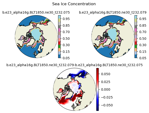
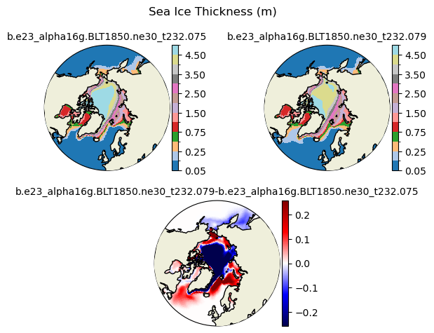
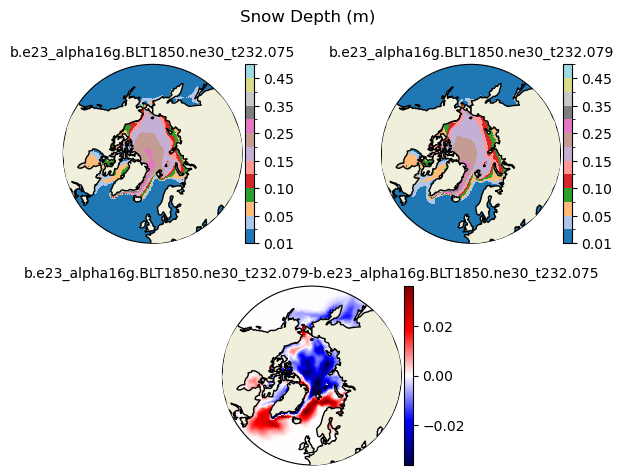
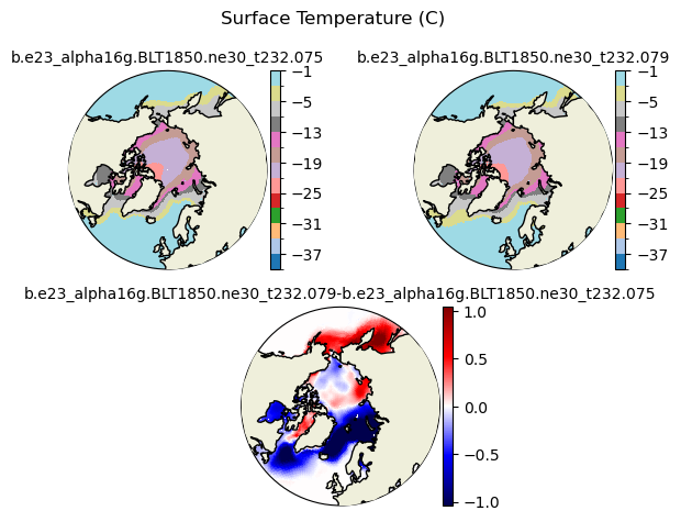
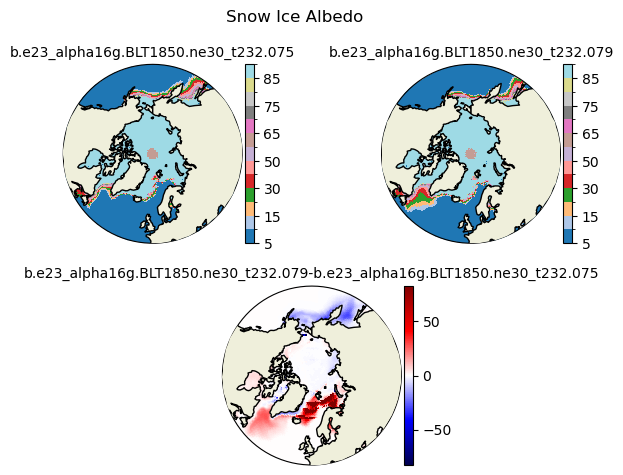
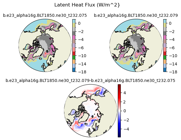
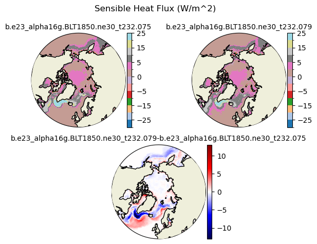
def plot_diff(field1, field2, levels, case1, case2, title, proj):
   # make circular boundary for polar stereographic circular plots
   theta = np.linspace(0, 2*np.pi, 100)
   center, radius = [0.5, 0.5], 0.5
   verts = np.vstack([np.sin(theta), np.cos(theta)]).T
   circle = mpath.Path(verts * radius + center)

   
   if (np.size(levels) > 2):
       cmap = mpl.colormaps['tab20']
       norm = mpl.colors.BoundaryNorm(levels, ncolors=cmap.N)

   # set up the figure with a North Polar Stereographic projection
   fig = plt.figure(tight_layout=True)
   gs = GridSpec(2, 4)

   if (proj == "N"):
      ax = fig.add_subplot(gs[0,:2], projection=ccrs.NorthPolarStereo())
      # sets the latitude / longitude boundaries of the plot
      ax.set_extent([0.005, 360, 90, 45], crs=ccrs.PlateCarree())
   if (proj == "S"):
      ax = fig.add_subplot(gs[0,:2], projection=ccrs.SouthPolarStereo())
      # sets the latitude / longitude boundaries of the plot
      ax.set_extent([0.005, 360, -90, -45], crs=ccrs.PlateCarree())

   ax.set_boundary(circle, transform=ax.transAxes)
   ax.add_feature(cfeature.LAND,zorder=100,edgecolor='k')

   field_diff = field2.values-field1.values
   field_std = field_diff.std()

   this=ax.pcolormesh(TLON,
                      TLAT,
                      field1,
                      norm = norm,
                      cmap="tab20",
                      transform=ccrs.PlateCarree())
   plt.colorbar(this,orientation='vertical',fraction=0.04,pad=0.01)
   plt.title(case1,fontsize=10)

   if (proj == "N"):
      ax = fig.add_subplot(gs[0,2:], projection=ccrs.NorthPolarStereo())
      # sets the latitude / longitude boundaries of the plot
      ax.set_extent([0.005, 360, 90, 45], crs=ccrs.PlateCarree())
   if (proj == "S"):
      ax = fig.add_subplot(gs[0,2:], projection=ccrs.SouthPolarStereo())
      # sets the latitude / longitude boundaries of the plot
      ax.set_extent([0.005, 360, -90, -45], crs=ccrs.PlateCarree())

   ax.set_boundary(circle, transform=ax.transAxes)
   ax.add_feature(cfeature.LAND,zorder=100,edgecolor='k')

   this=ax.pcolormesh(TLON,
                      TLAT,
                      field2,
                      norm=norm,
                      cmap="tab20",
                      transform=ccrs.PlateCarree())
   plt.colorbar(this,orientation='vertical',fraction=0.04,pad=0.01)
   plt.title(case2,fontsize=10)

   if (proj == "N"):
      ax = fig.add_subplot(gs[1,1:3], projection=ccrs.NorthPolarStereo())
      # sets the latitude / longitude boundaries of the plot
      ax.set_extent([0.005, 360, 90, 45], crs=ccrs.PlateCarree())
   if (proj == "S"):
      ax = fig.add_subplot(gs[1,1:3], projection=ccrs.SouthPolarStereo())
      # sets the latitude / longitude boundaries of the plot
      ax.set_extent([0.005, 360, -90, -45], crs=ccrs.PlateCarree())

   ax.set_boundary(circle, transform=ax.transAxes)
   ax.add_feature(cfeature.LAND,zorder=100,edgecolor='k')

   this=ax.pcolormesh(TLON,
                      TLAT,
                      field_diff,
                      cmap="seismic",vmax=field_std*2.0,vmin=-field_std*2.0,
                      transform=ccrs.PlateCarree())
   plt.colorbar(this,orientation='vertical',fraction=0.04,pad=0.01)
   plt.title(case2+"-"+case1,fontsize=10)

   plt.suptitle(title)

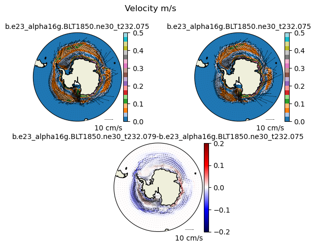
def vect_diff(uvel1,vvel1,uvel2,vvel2,angle,proj):
    uvel_rot1 = uvel1*np.cos(angle)-vvel1*np.sin(angle)
    vvel_rot1 = uvel1*np.sin(angle)+vvel1*np.cos(angle)
    uvel_rot2 = uvel2*np.cos(angle)-vvel2*np.sin(angle)
    vvel_rot2 = uvel2*np.sin(angle)+vvel2*np.cos(angle)
    
    speed1 = np.sqrt(uvel1*uvel1+vvel1*vvel1)
    speed2 = np.sqrt(uvel2*uvel2+vvel2*vvel2)

    uvel_diff = uvel_rot2-uvel_rot1
    vvel_diff = vvel_rot2-vvel_rot1
    speed_diff = speed2-speed1
    
    # make circular boundary for polar stereographic circular plots
    theta = np.linspace(0, 2*np.pi, 100)
    center, radius = [0.5, 0.5], 0.5
    verts = np.vstack([np.sin(theta), np.cos(theta)]).T
    circle = mpath.Path(verts * radius + center)

    # set up the figure with a North Polar Stereographic projection
    fig = plt.figure(tight_layout=True)
    gs = GridSpec(2, 4)

    if (proj == "N"):
       ax = fig.add_subplot(gs[0,:2], projection=ccrs.NorthPolarStereo())
       # sets the latitude / longitude boundaries of the plot
       ax.set_extent([0.005, 360, 90, 45], crs=ccrs.PlateCarree())
    if (proj == "S"):
       ax = fig.add_subplot(gs[0,:2], projection=ccrs.SouthPolarStereo())
       # sets the latitude / longitude boundaries of the plot
       ax.set_extent([0.005, 360, -90, -45], crs=ccrs.PlateCarree())

    ax.set_boundary(circle, transform=ax.transAxes)
    ax.add_feature(cfeature.LAND,zorder=100,edgecolor='k')

    this=ax.pcolormesh(TLON,
                     TLAT,
                     speed1,
                     vmin = 0.,
                     vmax = 0.5,
                     cmap="tab20",
                     transform=ccrs.PlateCarree())
    plt.colorbar(this,orientation='vertical',fraction=0.04,pad=0.01)
    plt.title(case1,fontsize=10)

    intv = 5
    ## add vectors
    Q = ax.quiver(TLON[::intv,::intv].values,TLAT[::intv,::intv].values,
                  uvel_rot1[::intv,::intv].values,vvel_rot1[::intv,::intv].values,
                  color = 'black', scale=1.,
                  transform=ccrs.PlateCarree())
    units = "cm/s"
    qk = ax.quiverkey(Q,0.85,0.025,0.10,r'10 '+units,labelpos='S', coordinates='axes',color='black',zorder=2)

    if (proj == "N"):
       ax = fig.add_subplot(gs[0,2:], projection=ccrs.NorthPolarStereo())
       # sets the latitude / longitude boundaries of the plot
       ax.set_extent([0.005, 360, 90, 45], crs=ccrs.PlateCarree())
    if (proj == "S"):
       ax = fig.add_subplot(gs[0,2:], projection=ccrs.SouthPolarStereo())
       # sets the latitude / longitude boundaries of the plot
       ax.set_extent([0.005, 360, -90, -45], crs=ccrs.PlateCarree())
        
    ax.set_boundary(circle, transform=ax.transAxes)
    ax.add_feature(cfeature.LAND,zorder=100,edgecolor='k')

    this=ax.pcolormesh(TLON,
                     TLAT,
                     speed2,
                     vmin = 0.,
                     vmax = 0.5,
                     cmap="tab20",
                     transform=ccrs.PlateCarree())
    plt.colorbar(this,orientation='vertical',fraction=0.04,pad=0.01)
    plt.title(case1,fontsize=10)

    intv = 5
    ## add vectors
    Q = ax.quiver(TLON[::intv,::intv].values,TLAT[::intv,::intv].values,
                  uvel_rot2[::intv,::intv].values,vvel_rot2[::intv,::intv].values,
                  color = 'black', scale=1.,
                  transform=ccrs.PlateCarree())
    units = "cm/s"
    qk = ax.quiverkey(Q,0.85,0.025,0.10,r'10 '+units,labelpos='S', coordinates='axes',color='black',zorder=2)

    if (proj == "N"):
       ax = fig.add_subplot(gs[1,1:3], projection=ccrs.NorthPolarStereo())
       # sets the latitude / longitude boundaries of the plot
       ax.set_extent([0.005, 360, 90, 45], crs=ccrs.PlateCarree())
    if (proj == "S"):
       ax = fig.add_subplot(gs[1,1:3], projection=ccrs.SouthPolarStereo())
       # sets the latitude / longitude boundaries of the plot
       ax.set_extent([0.005, 360, -90, -45], crs=ccrs.PlateCarree())
        
    ax.set_boundary(circle, transform=ax.transAxes)
    ax.add_feature(cfeature.LAND,zorder=100,edgecolor='k')

    this=ax.pcolormesh(TLON,
                     TLAT,
                     speed_diff,
                     vmin = -0.2,
                     vmax = 0.2,
                     cmap="seismic",
                     transform=ccrs.PlateCarree())
    plt.colorbar(this,orientation='vertical',fraction=0.04,pad=0.01)
    plt.title(case2+"-"+case1,fontsize=10)

    intv = 5
    ## add vectors
    Q = ax.quiver(TLON[::intv,::intv].values,TLAT[::intv,::intv].values,
                  uvel_diff[::intv,::intv].values,vvel_diff[::intv,::intv].values,
                  color = 'black', scale=1.,
                  transform=ccrs.PlateCarree())
    units = "cm/s"
    qk = ax.quiverkey(Q,0.85,0.025,0.10,r'10 '+units,labelpos='S', coordinates='axes',color='black',zorder=2)

    plt.suptitle("Velocity m/s")

with open('cice_vars.yml', 'r') as file:
    cice_vars = yaml.safe_load(file)


for var in cice_vars:
    print(var,cice_vars[var])
    vmin=cice_vars[var][0]['levels'][0]
    vmax=cice_vars[var][0]['levels'][-1]
    levels = np.array(cice_vars[var][0]['levels'])
    print(levels)
    title=cice_vars[var][1]['title']
    field1 = ds1_ann[var].isel(time=slice(-nyears,None)).mean("time").squeeze()
    field2 = ds2_ann[var].isel(time=slice(-nyears,None)).mean("time").squeeze()
    plot_diff(field1,field2,levels,case1,case2,title,"N")

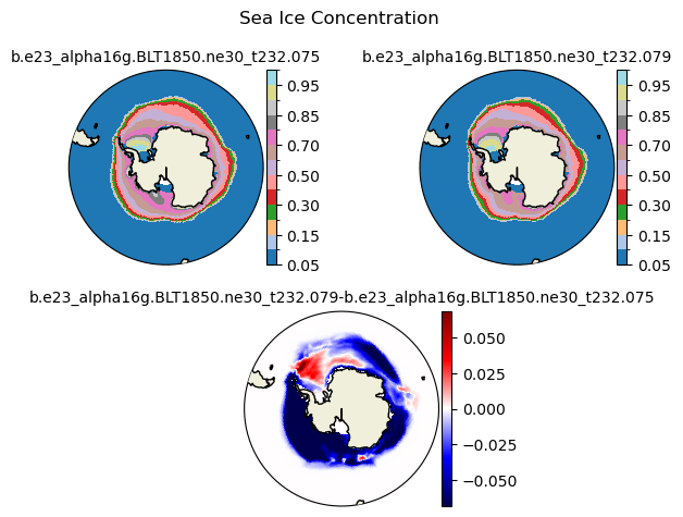
aice [{'levels': [0.05, 0.1, 0.15, 0.2, 0.3, 0.4, 0.5, 0.6, 0.7, 0.8, 0.85, 0.9, 0.95, 0.99]}, {'title': 'Sea Ice Concentration'}]
[0.05 0.1  0.15 0.2  0.3  0.4  0.5  0.6  0.7  0.8  0.85 0.9  0.95 0.99]

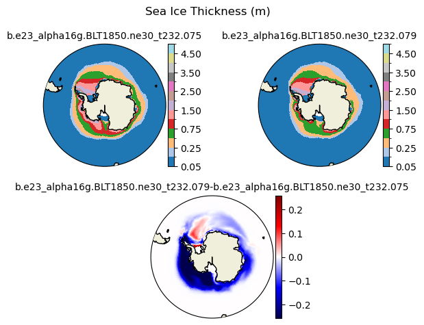
hi [{'levels': [0.05, 0.1, 0.25, 0.5, 0.75, 1.0, 1.5, 2.0, 2.5, 3.0, 3.5, 4.0, 4.5, 5.0]}, {'title': 'Sea Ice Thickness (m)'}]
[0.05 0.1  0.25 0.5  0.75 1.   1.5  2.   2.5  3.   3.5  4.   4.5  5.  ]

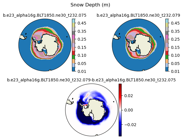
hs [{'levels': [0.01, 0.03, 0.05, 0.07, 0.1, 0.13, 0.15, 0.2, 0.25, 0.3, 0.35, 0.4, 0.45, 0.5]}, {'title': 'Snow Depth (m)'}]
[0.01 0.03 0.05 0.07 0.1  0.13 0.15 0.2  0.25 0.3  0.35 0.4  0.45 0.5 ]

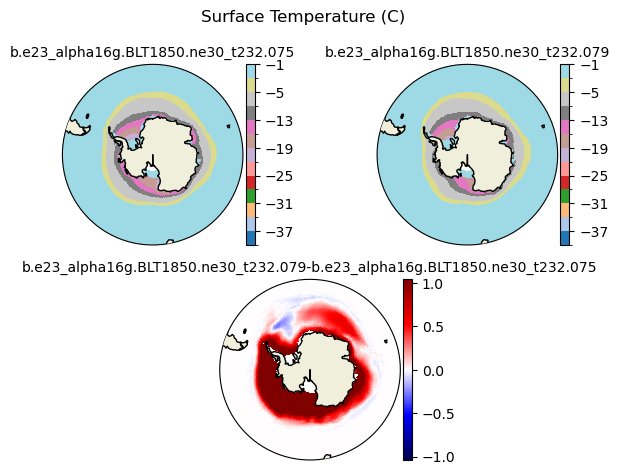
Tsfc [{'levels': [-40.0, -37.0, -34.0, -31.0, -28.0, -25.0, -22.0, -19.0, -16.0, -13.0, -10.0, -5.0, -3.0, -1.0]}, {'title': 'Surface Temperature (C)'}]
[-40. -37. -34. -31. -28. -25. -22. -19. -16. -13. -10.  -5.  -3.  -1.]

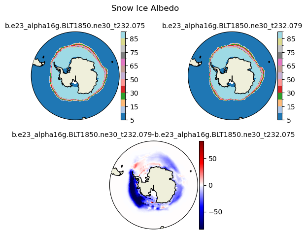
albsni [{'levels': [5, 10, 15, 20, 30, 40, 50, 60, 65, 70, 75, 80, 85, 90]}, {'title': 'Snow Ice Albedo'}]
[ 5 10 15 20 30 40 50 60 65 70 75 80 85 90]

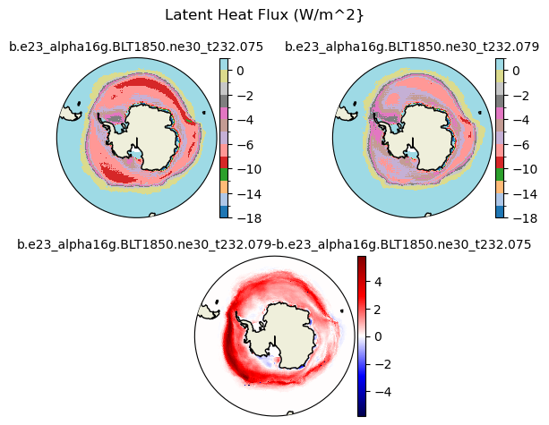
flat [{'levels': [-18.0, -16.0, -14.0, -12.0, -10.0, -8.0, -6.0, -5.0, -4.0, -3.0, -2.0, -1.0, 0.0, 2.0]}, {'title': 'Latent Heat Flux (W/m^2}'}]
[-18. -16. -14. -12. -10.  -8.  -6.  -5.  -4.  -3.  -2.  -1.   0.   2.]

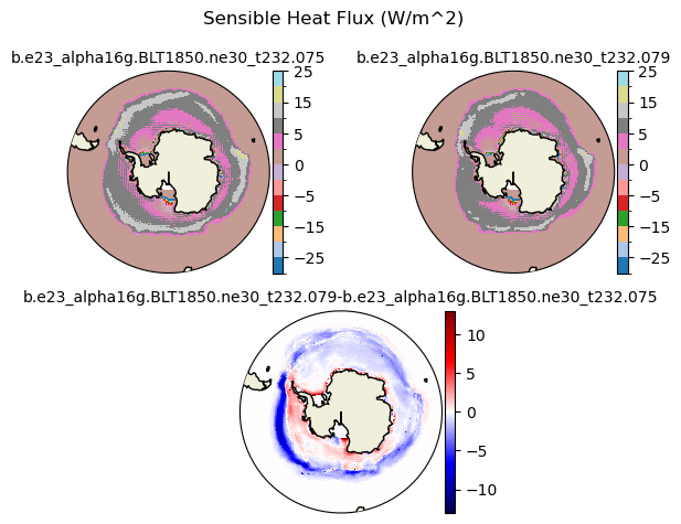
fsens [{'levels': [-30.0, -25.0, -20.0, -15.0, -10.0, -5.0, -2.5, 0, 2.5, 5, 10, 15, 20, 25]}, {'title': 'Sensible Heat Flux (W/m^2)'}]
[-30.  -25.  -20.  -15.  -10.   -5.   -2.5   0.    2.5   5.   10.   15.
  20.   25. ]

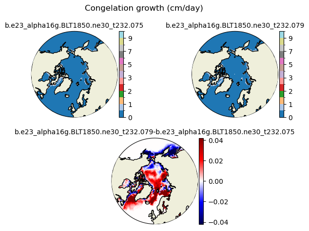
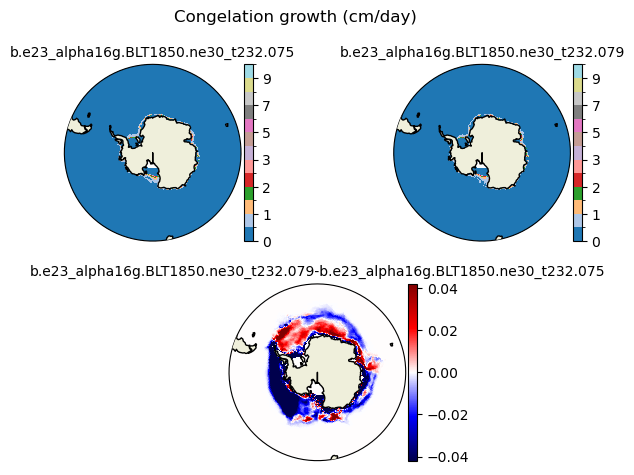
congel [{'levels': [0, 0.5, 1, 1.5, 2, 2.5, 3, 4, 5, 6, 7, 8, 9, 10]}, {'title': 'Congelation growth (cm/day)'}]
[ 0.   0.5  1.   1.5  2.   2.5  3.   4.   5.   6.   7.   8.   9.  10. ]

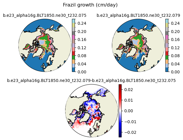
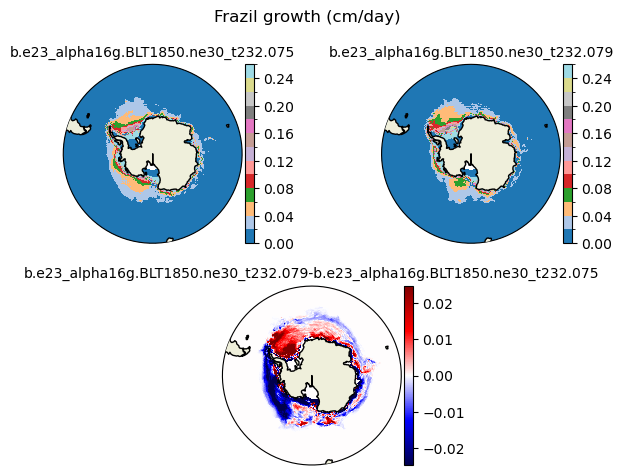
frazil [{'levels': [0.0, 0.02, 0.04, 0.06, 0.08, 0.1, 0.12, 0.14, 0.16, 0.18, 0.2, 0.22, 0.24, 0.26]}, {'title': 'Frazil growth (cm/day)'}]
[0.   0.02 0.04 0.06 0.08 0.1  0.12 0.14 0.16 0.18 0.2  0.22 0.24 0.26]

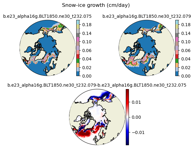
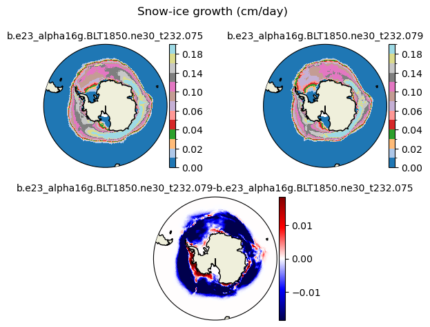
snoice [{'levels': [0.0, 0.01, 0.02, 0.03, 0.04, 0.05, 0.06, 0.08, 0.1, 0.12, 0.14, 0.16, 0.18, 0.2]}, {'title': 'Snow-ice growth (cm/day)'}]
[0.   0.01 0.02 0.03 0.04 0.05 0.06 0.08 0.1  0.12 0.14 0.16 0.18 0.2 ]

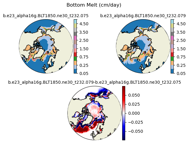
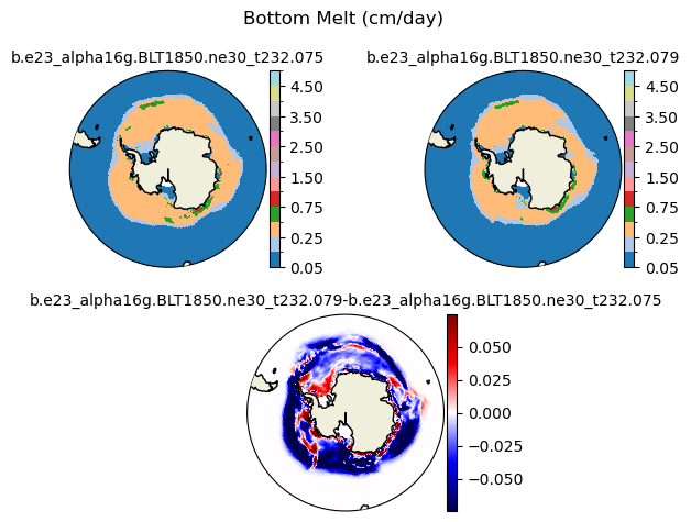
meltb [{'levels': [0.05, 0.1, 0.25, 0.5, 0.75, 1.0, 1.5, 2.0, 2.5, 3.0, 3.5, 4.0, 4.5, 5.0]}, {'title': 'Bottom Melt (cm/day)'}]
[0.05 0.1  0.25 0.5  0.75 1.   1.5  2.   2.5  3.   3.5  4.   4.5  5.  ]

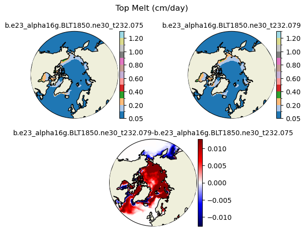
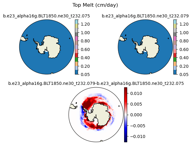
meltt [{'levels': [0.05, 0.1, 0.2, 0.3, 0.4, 0.5, 0.6, 0.7, 0.8, 0.9, 1.0, 1.1, 1.2, 1.3]}, {'title': 'Top Melt (cm/day)'}]
[0.05 0.1  0.2  0.3  0.4  0.5  0.6  0.7  0.8  0.9  1.   1.1  1.2  1.3 ]

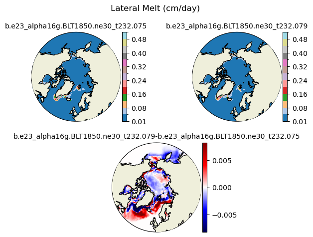
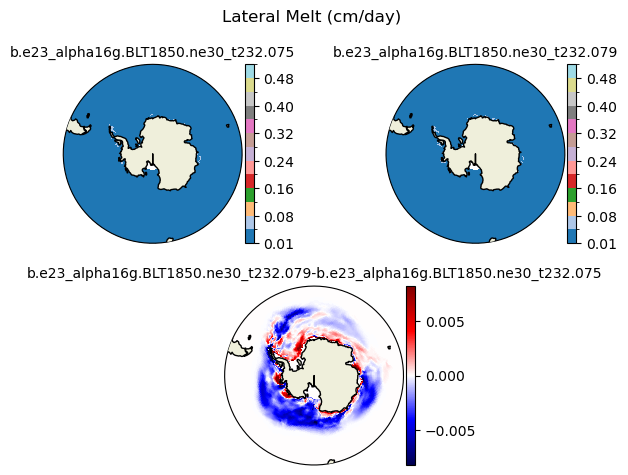
meltl [{'levels': [0.01, 0.04, 0.08, 0.12, 0.16, 0.2, 0.24, 0.28, 0.32, 0.36, 0.4, 0.44, 0.48, 0.52]}, {'title': 'Lateral Melt (cm/day)'}]
[0.01 0.04 0.08 0.12 0.16 0.2  0.24 0.28 0.32 0.36 0.4  0.44 0.48 0.52]

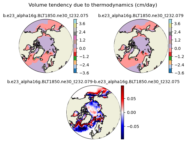
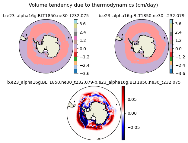
dvidtt [{'levels': [-3.6, -3.0, -2.4, -1.8, -1.2, -0.6, 0.0, 0.6, 1.2, 1.8, 2.4, 3.0, 3.6, 4.0]}, {'title': 'Volume tendency due to thermodynamics (cm/day)'}]
[-3.6 -3.  -2.4 -1.8 -1.2 -0.6  0.   0.6  1.2  1.8  2.4  3.   3.6  4. ]

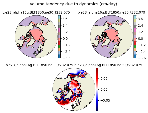
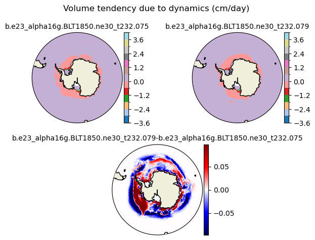
dvidtd [{'levels': [-3.6, -3.0, -2.4, -1.8, -1.2, -0.6, 0.0, 0.6, 1.2, 1.8, 2.4, 3.0, 3.6, 4.0]}, {'title': 'Volume tendency due to dynamics (cm/day)'}]
[-3.6 -3.  -2.4 -1.8 -1.2 -0.6  0.   0.6  1.2  1.8  2.4  3.   3.6  4. ]

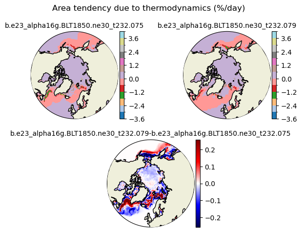
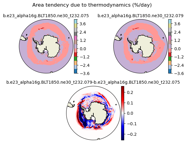
daidtt [{'levels': [-3.6, -3.0, -2.4, -1.8, -1.2, -0.6, 0.0, 0.6, 1.2, 1.8, 2.4, 3.0, 3.6, 4.0]}, {'title': 'Area tendency due to thermodynamics (%/day)'}]
[-3.6 -3.  -2.4 -1.8 -1.2 -0.6  0.   0.6  1.2  1.8  2.4  3.   3.6  4. ]

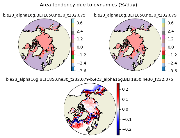
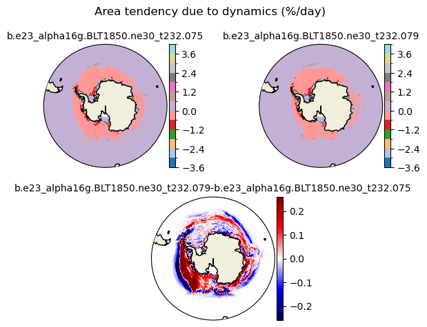
daidtd [{'levels': [-3.6, -3.0, -2.4, -1.8, -1.2, -0.6, 0.0, 0.6, 1.2, 1.8, 2.4, 3.0, 3.6, 4.0]}, {'title': 'Area tendency due to dynamics (%/day)'}]
[-3.6 -3.  -2.4 -1.8 -1.2 -0.6  0.   0.6  1.2  1.8  2.4  3.   3.6  4. ]

for var in cice_vars:
    print(var,cice_vars[var])
    vmin=cice_vars[var][0]['levels'][0]
    vmax=cice_vars[var][0]['levels'][1]
    levels = np.array(cice_vars[var][0]['levels'])
    print(levels)
    title=cice_vars[var][1]['title']
    field1 = ds1_ann[var].isel(time=slice(-nyears,None)).mean("time").squeeze()
    field2 = ds2_ann[var].isel(time=slice(-nyears,None)).mean("time").squeeze()
    plot_diff(field1,field2,levels,case1,case2,title,"S")

aice [{'levels': [0.05, 0.1, 0.15, 0.2, 0.3, 0.4, 0.5, 0.6, 0.7, 0.8, 0.85, 0.9, 0.95, 0.99]}, {'title': 'Sea Ice Concentration'}]
[0.05 0.1  0.15 0.2  0.3  0.4  0.5  0.6  0.7  0.8  0.85 0.9  0.95 0.99]

hi [{'levels': [0.05, 0.1, 0.25, 0.5, 0.75, 1.0, 1.5, 2.0, 2.5, 3.0, 3.5, 4.0, 4.5, 5.0]}, {'title': 'Sea Ice Thickness (m)'}]
[0.05 0.1  0.25 0.5  0.75 1.   1.5  2.   2.5  3.   3.5  4.   4.5  5.  ]

hs [{'levels': [0.01, 0.03, 0.05, 0.07, 0.1, 0.13, 0.15, 0.2, 0.25, 0.3, 0.35, 0.4, 0.45, 0.5]}, {'title': 'Snow Depth (m)'}]
[0.01 0.03 0.05 0.07 0.1  0.13 0.15 0.2  0.25 0.3  0.35 0.4  0.45 0.5 ]

Tsfc [{'levels': [-40.0, -37.0, -34.0, -31.0, -28.0, -25.0, -22.0, -19.0, -16.0, -13.0, -10.0, -5.0, -3.0, -1.0]}, {'title': 'Surface Temperature (C)'}]
[-40. -37. -34. -31. -28. -25. -22. -19. -16. -13. -10.  -5.  -3.  -1.]

albsni [{'levels': [5, 10, 15, 20, 30, 40, 50, 60, 65, 70, 75, 80, 85, 90]}, {'title': 'Snow Ice Albedo'}]
[ 5 10 15 20 30 40 50 60 65 70 75 80 85 90]

flat [{'levels': [-18.0, -16.0, -14.0, -12.0, -10.0, -8.0, -6.0, -5.0, -4.0, -3.0, -2.0, -1.0, 0.0, 2.0]}, {'title': 'Latent Heat Flux (W/m^2}'}]
[-18. -16. -14. -12. -10.  -8.  -6.  -5.  -4.  -3.  -2.  -1.   0.   2.]

fsens [{'levels': [-30.0, -25.0, -20.0, -15.0, -10.0, -5.0, -2.5, 0, 2.5, 5, 10, 15, 20, 25]}, {'title': 'Sensible Heat Flux (W/m^2)'}]
[-30.  -25.  -20.  -15.  -10.   -5.   -2.5   0.    2.5   5.   10.   15.
  20.   25. ]

congel [{'levels': [0, 0.5, 1, 1.5, 2, 2.5, 3, 4, 5, 6, 7, 8, 9, 10]}, {'title': 'Congelation growth (cm/day)'}]
[ 0.   0.5  1.   1.5  2.   2.5  3.   4.   5.   6.   7.   8.   9.  10. ]

frazil [{'levels': [0.0, 0.02, 0.04, 0.06, 0.08, 0.1, 0.12, 0.14, 0.16, 0.18, 0.2, 0.22, 0.24, 0.26]}, {'title': 'Frazil growth (cm/day)'}]
[0.   0.02 0.04 0.06 0.08 0.1  0.12 0.14 0.16 0.18 0.2  0.22 0.24 0.26]

snoice [{'levels': [0.0, 0.01, 0.02, 0.03, 0.04, 0.05, 0.06, 0.08, 0.1, 0.12, 0.14, 0.16, 0.18, 0.2]}, {'title': 'Snow-ice growth (cm/day)'}]
[0.   0.01 0.02 0.03 0.04 0.05 0.06 0.08 0.1  0.12 0.14 0.16 0.18 0.2 ]

meltb [{'levels': [0.05, 0.1, 0.25, 0.5, 0.75, 1.0, 1.5, 2.0, 2.5, 3.0, 3.5, 4.0, 4.5, 5.0]}, {'title': 'Bottom Melt (cm/day)'}]
[0.05 0.1  0.25 0.5  0.75 1.   1.5  2.   2.5  3.   3.5  4.   4.5  5.  ]

meltt [{'levels': [0.05, 0.1, 0.2, 0.3, 0.4, 0.5, 0.6, 0.7, 0.8, 0.9, 1.0, 1.1, 1.2, 1.3]}, {'title': 'Top Melt (cm/day)'}]
[0.05 0.1  0.2  0.3  0.4  0.5  0.6  0.7  0.8  0.9  1.   1.1  1.2  1.3 ]

meltl [{'levels': [0.01, 0.04, 0.08, 0.12, 0.16, 0.2, 0.24, 0.28, 0.32, 0.36, 0.4, 0.44, 0.48, 0.52]}, {'title': 'Lateral Melt (cm/day)'}]
[0.01 0.04 0.08 0.12 0.16 0.2  0.24 0.28 0.32 0.36 0.4  0.44 0.48 0.52]

dvidtt [{'levels': [-3.6, -3.0, -2.4, -1.8, -1.2, -0.6, 0.0, 0.6, 1.2, 1.8, 2.4, 3.0, 3.6, 4.0]}, {'title': 'Volume tendency due to thermodynamics (cm/day)'}]
[-3.6 -3.  -2.4 -1.8 -1.2 -0.6  0.   0.6  1.2  1.8  2.4  3.   3.6  4. ]

dvidtd [{'levels': [-3.6, -3.0, -2.4, -1.8, -1.2, -0.6, 0.0, 0.6, 1.2, 1.8, 2.4, 3.0, 3.6, 4.0]}, {'title': 'Volume tendency due to dynamics (cm/day)'}]
[-3.6 -3.  -2.4 -1.8 -1.2 -0.6  0.   0.6  1.2  1.8  2.4  3.   3.6  4. ]

daidtt [{'levels': [-3.6, -3.0, -2.4, -1.8, -1.2, -0.6, 0.0, 0.6, 1.2, 1.8, 2.4, 3.0, 3.6, 4.0]}, {'title': 'Area tendency due to thermodynamics (%/day)'}]
[-3.6 -3.  -2.4 -1.8 -1.2 -0.6  0.   0.6  1.2  1.8  2.4  3.   3.6  4. ]

daidtd [{'levels': [-3.6, -3.0, -2.4, -1.8, -1.2, -0.6, 0.0, 0.6, 1.2, 1.8, 2.4, 3.0, 3.6, 4.0]}, {'title': 'Area tendency due to dynamics (%/day)'}]
[-3.6 -3.  -2.4 -1.8 -1.2 -0.6  0.   0.6  1.2  1.8  2.4  3.   3.6  4. ]

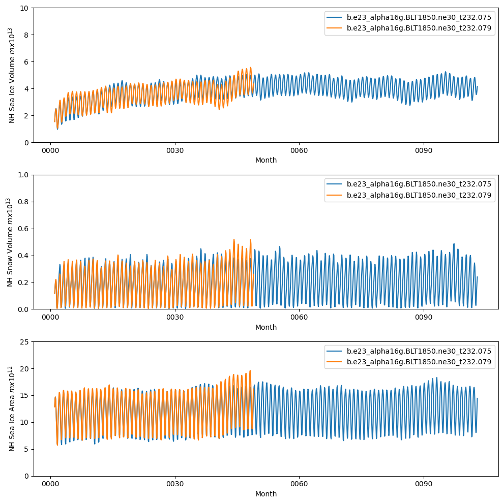
ds1_area = (tarea*ds1.aice).where(TLAT>0).sum(dim=['nj','ni'])*1.0e-12
ds2_area = (tarea*ds2.aice).where(TLAT>0).sum(dim=['nj','ni'])*1.0e-12

ds1_vhi = (tarea*ds1.hi).where(TLAT>0).sum(dim=['nj','ni'])*1.0e-13
ds2_vhi = (tarea*ds2.hi).where(TLAT>0).sum(dim=['nj','ni'])*1.0e-13

ds1_vhs = (tarea*ds1.hs).where(TLAT>0).sum(dim=['nj','ni'])*1.0e-13
ds2_vhs = (tarea*ds2.hs).where(TLAT>0).sum(dim=['nj','ni'])*1.0e-13

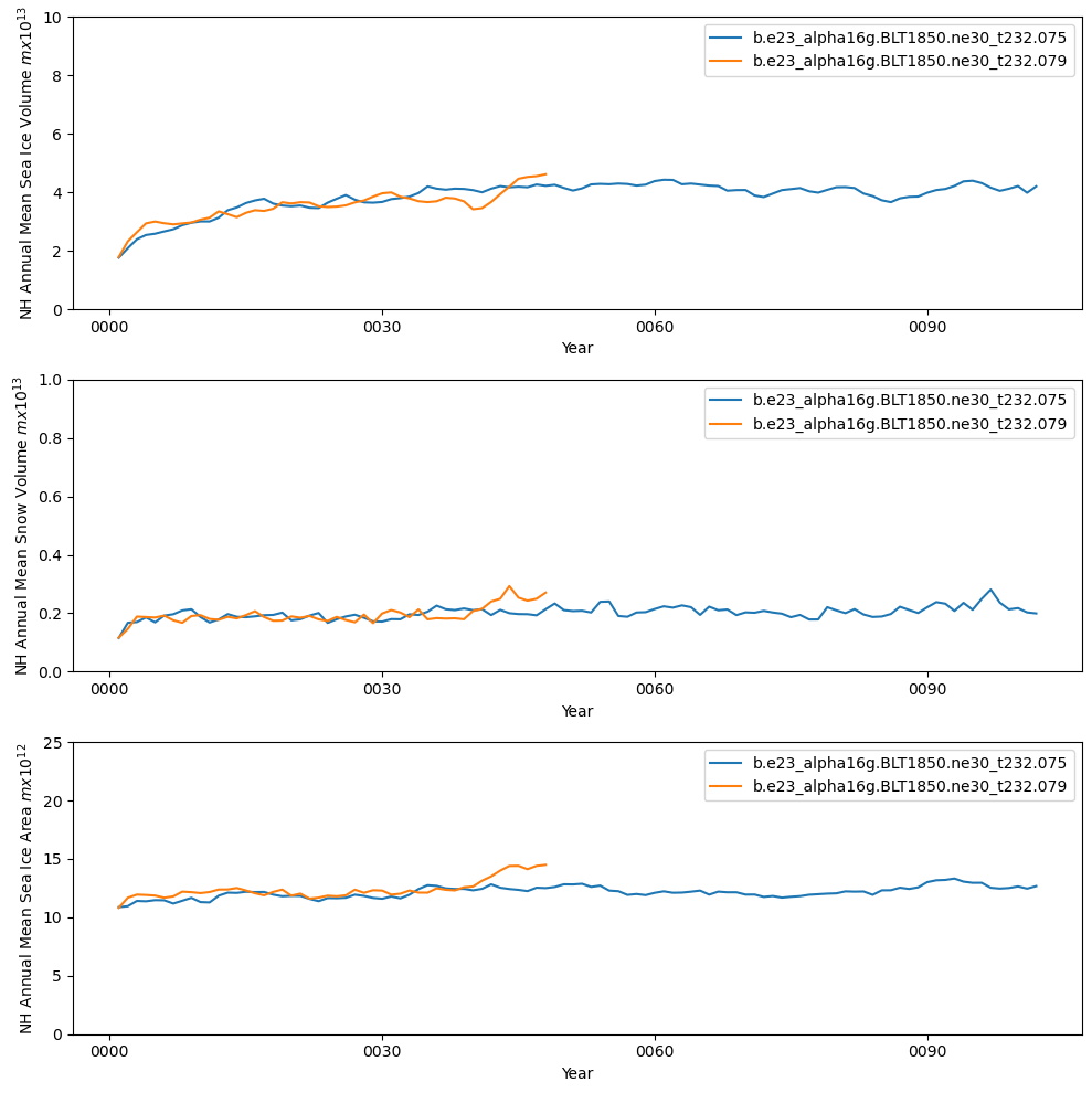
fig = plt.figure(figsize=(10,10),tight_layout=True)

ax = fig.add_subplot(3,1,1)
ds1_vhi.plot()
ds2_vhi.plot()

plt.ylim((0,10))
plt.xlabel("Month")
plt.ylabel("NH Sea Ice Volume $m x 10^{13}$")
plt.legend([case1,case2])

ax = fig.add_subplot(3,1,2)
ds1_vhs.plot()
ds2_vhs.plot()

plt.ylim((0,1))
plt.xlabel("Month")
plt.ylabel("NH Snow Volume $m x 10^{13}$")
plt.legend([case1,case2])

ax = fig.add_subplot(3,1,3)
ds1_area.plot()
ds2_area.plot()

plt.ylim((0,25))
plt.xlabel("Month")
plt.ylabel("NH Sea Ice Area $m x 10^{12}$")
plt.legend([case1,case2])

<matplotlib.legend.Legend at 0x7fbad6bf8190>

ds1_area_ann = (tarea*ds1_ann['aice']).where(TLAT>0).sum(dim=['nj','ni'])*1.0e-12
ds2_area_ann = (tarea*ds2_ann['aice']).where(TLAT>0).sum(dim=['nj','ni'])*1.0e-12

ds1_vhi_ann = (tarea*ds1_ann['hi']).where(TLAT>0).sum(dim=['nj','ni'])*1.0e-13
ds2_vhi_ann = (tarea*ds2_ann['hi']).where(TLAT>0).sum(dim=['nj','ni'])*1.0e-13

ds1_vhs_ann = (tarea*ds1_ann['hs']).where(TLAT>0).sum(dim=['nj','ni'])*1.0e-13
ds2_vhs_ann = (tarea*ds2_ann['hs']).where(TLAT>0).sum(dim=['nj','ni'])*1.0e-13

fig = plt.figure(figsize=(10,10),tight_layout=True)

ax = fig.add_subplot(3,1,1)
ds1_vhi_ann.plot()
ds2_vhi_ann.plot()

plt.ylim((0,10))
plt.xlabel("Year")
plt.ylabel("NH Annual Mean Sea Ice Volume $m x 10^{13}$")
plt.legend([case1,case2])

ax = fig.add_subplot(3,1,2)
ds1_vhs_ann.plot()
ds2_vhs_ann.plot()

plt.ylim((0,1))
plt.xlabel("Year")
plt.ylabel("NH Annual Mean Snow Volume $m x 10^{13}$")
plt.legend([case1,case2])

ax = fig.add_subplot(3,1,3)
ds1_area_ann.plot()
ds2_area_ann.plot()

plt.ylim((0,25))
plt.xlabel("Year")
plt.ylabel("NH Annual Mean Sea Ice Area $m x 10^{12}$")
plt.legend([case1,case2])

<matplotlib.legend.Legend at 0x7fbadb201610>

ds1_area.sel(time=ds1_area.time.dt.month.isin([10])).plot() ds2_area.sel(time=ds2_area.time.dt.month.isin([10])).plot()

plt.ylim((0,25)) plt.xlabel(“Year”) plt.ylabel(“NH September Sea Ice Area \(m x 10^{12}\)”) plt.legend([case1,case2])

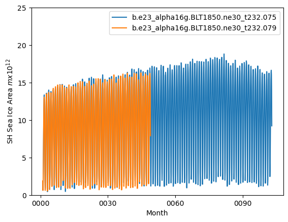
ds1_area = (tarea*ds1.aice).where(TLAT<0).sum(dim=['nj','ni'])*1.0e-12
ds2_area = (tarea*ds2.aice).where(TLAT<0).sum(dim=['nj','ni'])*1.0e-12

ds1_area.plot()
ds2_area.plot()

plt.ylim((0,25))
plt.xlabel("Month")
plt.ylabel("SH Sea Ice Area $m x 10^{12}$")
plt.legend([case1,case2])

<matplotlib.legend.Legend at 0x7fbaf9399610>

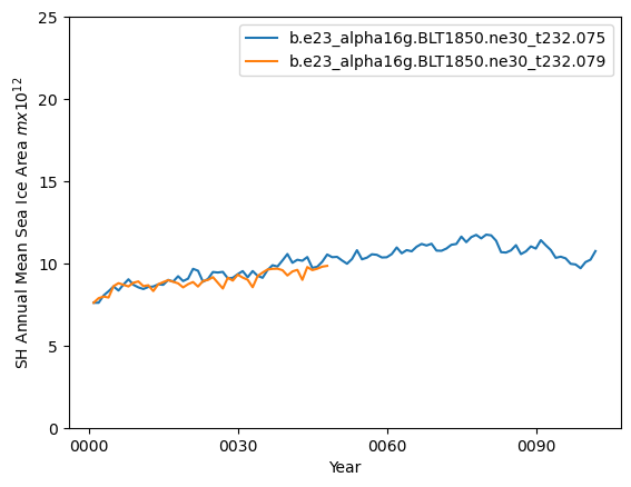
ds1_area_ann = (tarea*ds1_ann.aice).where(TLAT<0).sum(dim=['nj','ni'])*1.0e-12
ds2_area_ann = (tarea*ds2_ann.aice).where(TLAT<0).sum(dim=['nj','ni'])*1.0e-12

ds1_area_ann.plot()
ds2_area_ann.plot()

plt.ylim((0,25))
plt.xlabel("Year")
plt.ylabel("SH Annual Mean Sea Ice Area $m x 10^{12}$")
plt.legend([case1,case2])

<matplotlib.legend.Legend at 0x7fbadc1b3f50>

### Read in the NSIDC data from files

path_nsidc = '/glade/campaign/cesm/development/pcwg/ice/data/NSIDC_SeaIce_extent/'

jan_nsidc = pd.read_csv(path_nsidc+'N_01_extent_v3.0.csv',na_values=['-99.9'])
feb_nsidc = pd.read_csv(path_nsidc+'N_02_extent_v3.0.csv',na_values=['-99.9'])
mar_nsidc = pd.read_csv(path_nsidc+'N_03_extent_v3.0.csv',na_values=['-99.9'])
apr_nsidc = pd.read_csv(path_nsidc+'N_04_extent_v3.0.csv',na_values=['-99.9'])
may_nsidc = pd.read_csv(path_nsidc+'N_05_extent_v3.0.csv',na_values=['-99.9'])
jun_nsidc = pd.read_csv(path_nsidc+'N_06_extent_v3.0.csv',na_values=['-99.9'])
jul_nsidc = pd.read_csv(path_nsidc+'N_07_extent_v3.0.csv',na_values=['-99.9'])
aug_nsidc = pd.read_csv(path_nsidc+'N_08_extent_v3.0.csv',na_values=['-99.9'])
sep_nsidc = pd.read_csv(path_nsidc+'N_09_extent_v3.0.csv',na_values=['-99.9'])
oct_nsidc = pd.read_csv(path_nsidc+'N_10_extent_v3.0.csv',na_values=['-99.9'])
nov_nsidc = pd.read_csv(path_nsidc+'N_11_extent_v3.0.csv',na_values=['-99.9'])
dec_nsidc = pd.read_csv(path_nsidc+'N_12_extent_v3.0.csv',na_values=['-99.9'])

jan_area = jan_nsidc.iloc[:,5].values
feb_area = feb_nsidc.iloc[:,5].values
mar_area = mar_nsidc.iloc[:,5].values
apr_area = apr_nsidc.iloc[:,5].values
may_area = may_nsidc.iloc[:,5].values
jun_area = jun_nsidc.iloc[:,5].values
jul_area = jul_nsidc.iloc[:,5].values
aug_area = aug_nsidc.iloc[:,5].values
sep_area = sep_nsidc.iloc[:,5].values
oct_area = oct_nsidc.iloc[:,5].values
nov_area = nov_nsidc.iloc[:,5].values
dec_area = dec_nsidc.iloc[:,5].values

jan_ext = jan_nsidc.iloc[:,4].values
feb_ext = feb_nsidc.iloc[:,4].values
mar_ext = mar_nsidc.iloc[:,4].values
apr_ext = apr_nsidc.iloc[:,4].values
may_ext = may_nsidc.iloc[:,4].values
jun_ext = jun_nsidc.iloc[:,4].values
jul_ext = jul_nsidc.iloc[:,4].values
aug_ext = aug_nsidc.iloc[:,4].values
sep_ext = sep_nsidc.iloc[:,4].values
oct_ext = oct_nsidc.iloc[:,4].values
nov_ext = nov_nsidc.iloc[:,4].values
dec_ext = dec_nsidc.iloc[:,4].values

print(dec_ext)
nsidc_clim = [np.nanmean(jan_ext[0:35]),np.nanmean(feb_ext[0:35]),np.nanmean(mar_ext[0:35]),np.nanmean(apr_ext[0:35]),
              np.nanmean(may_ext[0:35]),np.nanmean(jun_ext[0:35]),np.nanmean(jul_ext[0:35]),np.nanmean(aug_ext[0:35]),
              np.nanmean(sep_ext[0:35]),np.nanmean(oct_ext[0:35]),np.nanmean(nov_ext[0:35]),np.nanmean(dec_ext[0:35])]

plt.plot(nsidc_clim)

[13.67 13.34 13.59 13.34 13.64 13.3  12.99 13.05 13.22   nan 13.63 13.39
 13.11 12.95 13.41 13.32 13.27 12.92 12.86 13.08 12.76 12.64 12.64 12.49
 12.61 12.59 12.55 12.23 11.95 12.03 12.36 12.2  11.83 12.15 12.01 12.18
 12.35 12.04 11.46 11.74 11.86]

[<matplotlib.lines.Line2D at 0x7fbade150350>]

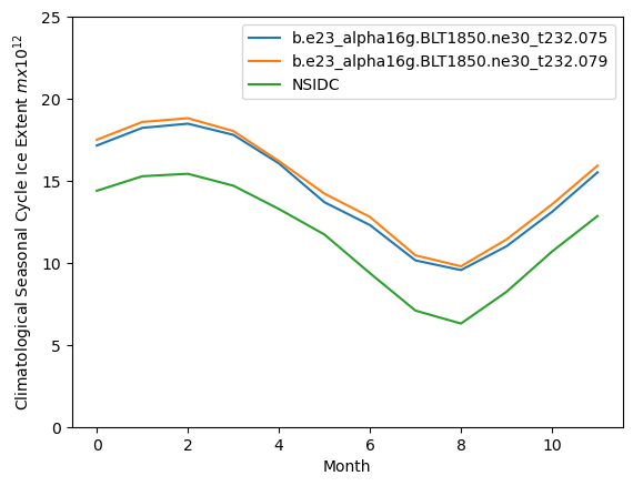
aice1_month = ds1['aice'].groupby("time.month").mean(dim="time",skipna=True)
aice2_month = ds2['aice'].groupby("time.month").mean(dim="time",skipna=True)

mask_tmp1 = np.where(np.logical_and(aice1_month > 0.15, ds1['TLAT'] > 0), 1., 0.)
mask_tmp2 = np.where(np.logical_and(aice2_month > 0.15, ds1['TLAT'] > 0), 1., 0.)

mask_ext1 = xr.DataArray(data=mask_tmp1,dims=["month","nj", "ni"])
mask_ext2 = xr.DataArray(data=mask_tmp2,dims=["month","nj", "ni"])


ext1 = (mask_ext1*tarea).sum(['ni','nj'])*1.0e-12
ext2 = (mask_ext2*tarea).sum(['ni','nj'])*1.0e-12

plt.plot(ext1)
plt.plot(ext2)
plt.plot(nsidc_clim)

plt.ylim((0,25))
plt.xlabel("Month")
plt.ylabel("Climatological Seasonal Cycle Ice Extent $m x 10^{12}$")
plt.legend([case1,case2,"NSIDC"])

/glade/work/dbailey/conda-envs/cupid-analysis/lib/python3.11/site-packages/distributed/client.py:3162: UserWarning: Sending large graph of size 24.99 MiB.
This may cause some slowdown.
Consider scattering data ahead of time and using futures.
  warnings.warn(

<matplotlib.legend.Legend at 0x7fbade302e10>

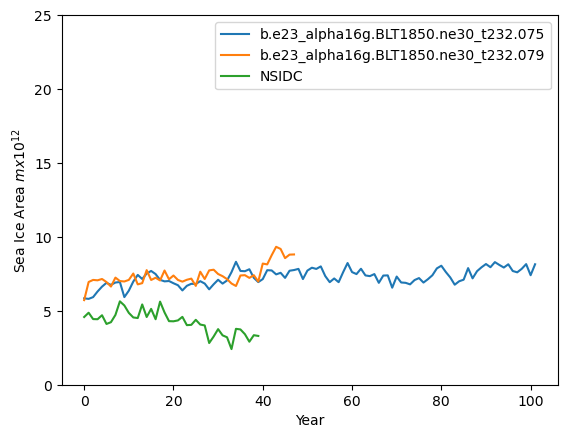
ds1_area = (tarea*ds1.aice).where(TLAT>0).sum(dim=['nj','ni'])*1.0e-12
ds2_area = (tarea*ds2.aice).where(TLAT>0).sum(dim=['nj','ni'])*1.0e-12

ds1_sep = ds1_area.sel(time=(ds1_area.time.dt.month == 9))
ds2_sep = ds2_area.sel(time=(ds2_area.time.dt.month == 9))

plt.plot(ds1_sep)
plt.plot(ds2_sep)
plt.plot(sep_area)

plt.ylim((0,25))
plt.xlabel("Year")
plt.ylabel("Sea Ice Area $mx10^{12}$")
plt.legend([case1,case2,"NSIDC"])

<matplotlib.legend.Legend at 0x7fbabfaf3490>

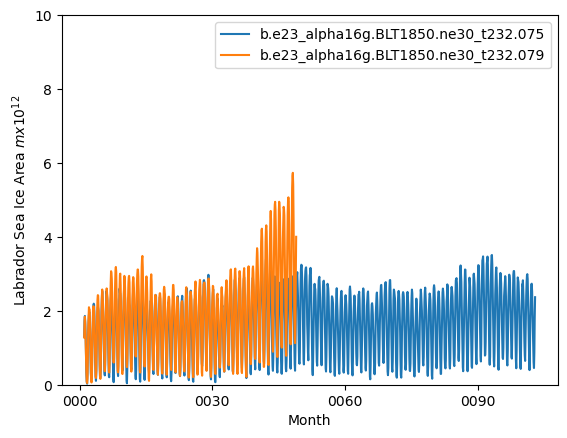
latm = cice_masks['Lab_lat']
lonm = cice_masks['Lab_lon']

lon = np.where(TLON < 0, TLON+360.,TLON)

mask1 = np.where(np.logical_and(TLAT > latm[0], TLAT < latm[1]),1.,0.)
mask2 = np.where(np.logical_or(lon > lonm[0], lon < lonm[1]),1.,0.)
mask = mask1*mask2

ds1_lab = (mask*tarea*ds1.aice).sum(dim=['nj','ni'])*1.0e-12
ds2_lab = (mask*tarea*ds2.aice).sum(dim=['nj','ni'])*1.0e-12

ds1_lab.plot()
ds2_lab.plot()

plt.ylim((0,10))
plt.xlabel("Month")
plt.ylabel("Labrador Sea Ice Area $m x 10^{12}$")
plt.legend([case1,case2])

<matplotlib.legend.Legend at 0x7fbade16ba90>

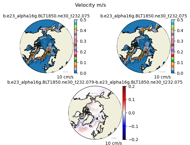
uvel1 = ds1_ann['uvel'].isel(time=slice(-nyears,None)).mean("time").squeeze()
vvel1 = ds1_ann['vvel'].isel(time=slice(-nyears,None)).mean("time").squeeze()
uvel2 = ds2_ann['uvel'].isel(time=slice(-nyears,None)).mean("time").squeeze()
vvel2 = ds2_ann['vvel'].isel(time=slice(-nyears,None)).mean("time").squeeze()
ds_angle = xr.open_dataset("/glade/derecho/scratch/dbailey/ADF/b.e23_alpha16g.BLT1850.ne30_t232.075c/ts/angle.nc")
angle = ds_angle['ANGLE']

vect_diff(uvel1,vvel1,uvel2,vvel2,angle,"N")

vect_diff(uvel1,vvel1,uvel2,vvel2,angle,"S")