Central America Globe Temperate North America

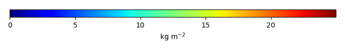
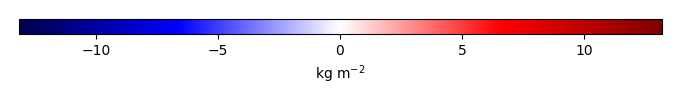
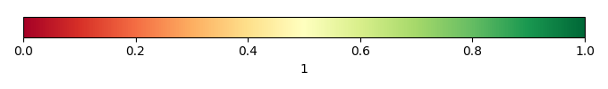
	Download Data	Period Mean (original grids) [Pg]	Model Period Mean (intersection) [Pg]	Model Period Mean (complement) [Pg]	Benchmark Period Mean (intersection) [Pg]	Benchmark Period Mean (complement) [Pg]		Bias [kg m-2]		Bias Score [1]	Spatial Distribution Score [1]	Overall Score [1]
Benchmark	[-]	0.797
CRUNCEPv7	[-]	10.2	0.768	9.20	0.538	0.0190		1.59		0.52	0.68	0.60
GSWP3v1	[-]	8.57	0.459	7.91	0.538	0.0190		0.552		0.57	0.78	0.68
WATCH	[-]	9.34	0.609	8.60	0.538	0.0190		0.967		0.59	0.76	0.68

	Download Data	Period Mean (original grids) [Pg]	Model Period Mean (intersection) [Pg]	Model Period Mean (complement) [Pg]	Benchmark Period Mean (intersection) [Pg]	Benchmark Period Mean (complement) [Pg]		Bias [kg m-2]		Bias Score [1]	Spatial Distribution Score [1]	Overall Score [1]
Benchmark	[-]	26.2
CRUNCEPv7	[-]	589.	21.7	567.	26.1	0.0878		-0.243		0.62	0.87	0.74
GSWP3v1	[-]	487.	15.3	472.	26.1	0.0878		-1.07		0.60	0.79	0.69
WATCH	[-]	505.	17.4	488.	26.1	0.0878		-0.829		0.63	0.81	0.72

	Download Data	Period Mean (original grids) [Pg]	Model Period Mean (intersection) [Pg]	Model Period Mean (complement) [Pg]	Benchmark Period Mean (intersection) [Pg]	Benchmark Period Mean (complement) [Pg]		Bias [kg m-2]		Bias Score [1]	Spatial Distribution Score [1]	Overall Score [1]
Benchmark	[-]	25.4
CRUNCEPv7	[-]	35.4	21.0	14.0	25.6	0.0688		-0.351		0.62	0.88	0.75
GSWP3v1	[-]	24.4	14.8	9.24	25.6	0.0688		-1.17		0.60	0.79	0.69
WATCH	[-]	25.1	16.8	8.05	25.6	0.0688		-0.934		0.63	0.80	0.72

Australia Boreal Asia Boreal North America Central America Central Asia Equatorial Asia Europe Globe Middle East Northern Hemisphere Africa Northern Hemisphere South America Southeast Asia Southern Hemisphere Africa Southern Hemisphere South America Temperate North America Temporally integrated period mean Temporally integrated period mean bias Temporally integrated period mean bias score

  Approach: To convert the original data at 250m to the final one at 0.5x0.5 degree resolution, Please see conversion steps listed in http://redwood.ess.uci.edu/mingquan/www/ILAMB/Download/CODES/CODES/subroutines/convert/readme_biomass. 3 codes below will be used in these steps. Code 1: http://redwood.ess.uci.edu/mingquan/www/ILAMB/Download/CODES/CODES/subroutines/convert/read-NBCD2000.pro Code 2: http://redwood.ess.uci.edu/mingquan/www/ILAMB/Download/CODES/CODES/subroutines/convert/convert-NBCD2000.ncl Code 3: http://redwood.ess.uci.edu/mingquan/www/ILAMB/Download/CODES/CODES/subroutines/convert/write-NBCD2000.ncl First, I used Code 1 to read data at 250m from the original geotiff file; then I used Code 2 to convert unit from the orignal unit of ton C per hectare to the final one of Kg C per m2, meanwhile I summed all available data points at 250m in each 0.5x0.5 grid cell to obtain the data at 0.5x0.5 degree resolution; finally I used Code 3 to create the final file in netCDF format.

  Temporal resolution: yearly

  General information: This product was derived from National Biomass and Carbon Dataset for the year 2000 originally in a raster format at 250m.

  Spatial resolution: 0.5x0.5 degree

  Derived data code: http://redwood.ess.uci.edu/mingquan/www/ILAMB/Download/CODES/CODES/subroutines/convert/read-NBCD2000.pro http://redwood.ess.uci.edu/mingquan/www/ILAMB/Download/CODES/CODES/subroutines/convert/convert-NBCD2000.ncl http://redwood.ess.uci.edu/mingquan/www/ILAMB/Download/CODES/CODES/subroutines/convert/write-NBCD2000.ncl