Globe North America - Alaska and Northern Canada North America - Central America North America - Eastern United States North America - Southern Canada North America - Western United States

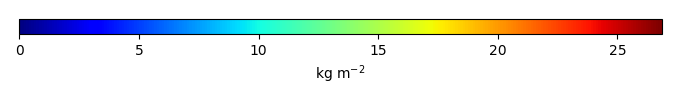
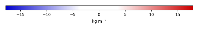
	Download Data	Period Mean (original grids) [Pg]	Model Period Mean (intersection) [Pg]	Model Period Mean (complement) [Pg]	Benchmark Period Mean (intersection) [Pg]	Benchmark Period Mean (complement) [Pg]		Bias [kg m-2]		Bias Score [1]	Spatial Distribution Score [1]	Overall Score [1]
Benchmark	[-]	30.1
CESM2_1	[-]	487.	16.4	470.	29.9	0.195		-1.17		0.538	0.679	0.609
CRUJRA	[-]	626.	29.3	597.	29.9	0.195		0.327		0.605	0.837	0.721
GSWP3	[-]	491.	22.4	468.	29.9	0.195		-0.472		0.574	0.772	0.673
PRINCETON	[-]	714.	35.9	678.	29.9	0.195		1.05		0.624	0.845	0.735

	Download Data	Period Mean (original grids) [Pg]	Model Period Mean (intersection) [Pg]	Model Period Mean (complement) [Pg]	Benchmark Period Mean (intersection) [Pg]	Benchmark Period Mean (complement) [Pg]		Bias [kg m-2]		Bias Score [1]	Spatial Distribution Score [1]	Overall Score [1]
Benchmark	[-]	1.44
CESM2_1	[-]	10.0	4.41	5.87	1.41	0.0279		2.74		0.350	0.574	0.462
CRUJRA	[-]	16.4	6.21	10.1	1.41	0.0279		4.48		0.202	0.428	0.315
GSWP3	[-]	14.9	6.04	8.72	1.41	0.0279		4.24		0.200	0.465	0.333
PRINCETON	[-]	22.3	7.89	14.4	1.41	0.0279		5.90		0.131	0.239	0.185

	Download Data	Period Mean (original grids) [Pg]	Model Period Mean (intersection) [Pg]	Model Period Mean (complement) [Pg]	Benchmark Period Mean (intersection) [Pg]	Benchmark Period Mean (complement) [Pg]		Bias [kg m-2]		Bias Score [1]	Spatial Distribution Score [1]	Overall Score [1]
Benchmark	[-]	0.00649
CESM2_1	[-]	9.84	0.0204	9.59	0.00649			0.164		0.488	0.577	0.532
CRUJRA	[-]	12.4	0.0314	12.1	0.00649			0.346		0.598	0.779	0.688
GSWP3	[-]	10.2	0.0247	9.96	0.00649			0.231		0.589	0.761	0.675
PRINCETON	[-]	13.7	0.0259	13.4	0.00649			0.253		0.586	0.761	0.673

	Download Data	Period Mean (original grids) [Pg]	Model Period Mean (intersection) [Pg]	Model Period Mean (complement) [Pg]	Benchmark Period Mean (intersection) [Pg]	Benchmark Period Mean (complement) [Pg]		Bias [kg m-2]		Bias Score [1]	Spatial Distribution Score [1]	Overall Score [1]
Benchmark	[-]	17.4
CESM2_1	[-]	9.53	9.25	0.198	17.3	0.0180		-1.66		0.605	0.845	0.725
CRUJRA	[-]	18.0	17.6	0.300	17.3	0.0180		0.471		0.703	0.930	0.816
GSWP3	[-]	11.9	11.6	0.244	17.3	0.0180		-1.07		0.648	0.854	0.751
PRINCETON	[-]	19.2	18.7	0.319	17.3	0.0180		0.762		0.695	0.925	0.810

	Download Data	Period Mean (original grids) [Pg]	Model Period Mean (intersection) [Pg]	Model Period Mean (complement) [Pg]	Benchmark Period Mean (intersection) [Pg]	Benchmark Period Mean (complement) [Pg]		Bias [kg m-2]		Bias Score [1]	Spatial Distribution Score [1]	Overall Score [1]
Benchmark	[-]	1.52
CESM2_1	[-]	35.2	1.15	33.8	1.46	0.0621		0.725		0.636	0.826	0.731
CRUJRA	[-]	53.4	2.12	51.3	1.46	0.0621		5.19		0.612	0.905	0.759
GSWP3	[-]	44.5	1.76	42.9	1.46	0.0621		3.57		0.645	0.899	0.772
PRINCETON	[-]	67.0	2.48	64.6	1.46	0.0621		6.90		0.586	0.902	0.744

	Download Data	Period Mean (original grids) [Pg]	Model Period Mean (intersection) [Pg]	Model Period Mean (complement) [Pg]	Benchmark Period Mean (intersection) [Pg]	Benchmark Period Mean (complement) [Pg]		Bias [kg m-2]		Bias Score [1]	Spatial Distribution Score [1]	Overall Score [1]
Benchmark	[-]	9.78
CESM2_1	[-]	1.65	1.56	0.118	9.71	0.0683		-2.12		0.429	0.208	0.318
CRUJRA	[-]	3.44	3.31	0.178	9.71	0.0683		-1.61		0.488	0.532	0.510
GSWP3	[-]	3.12	3.01	0.149	9.71	0.0683		-1.71		0.483	0.415	0.449
PRINCETON	[-]	6.93	6.74	0.219	9.71	0.0683		-0.669		0.574	0.785	0.679

Africa - Central Africa - Sahel Africa - South Asia - East Siberia Asia - Indonesia Asia - North Central Asia - South Central Asia and China Asia - Southeast Asia and India Asia - West Siberia Australia Europe Globe Middle East and Sahara North America - Alaska and Northern Canada North America - Central America North America - Eastern United States North America - Southern Canada North America - Western United States South America - Amazon South America - Southeast South America - Southwest Temporally integrated period mean Temporally integrated period mean bias Temporally integrated period mean bias score

  Approach: To convert the original data at 250m to the final one at 0.5x0.5 degree resolution, Please see conversion steps listed in http://redwood.ess.uci.edu/mingquan/www/ILAMB/Download/CODES/CODES/subroutines/convert/readme_biomass. 3 codes below will be used in these steps. Code 1: http://redwood.ess.uci.edu/mingquan/www/ILAMB/Download/CODES/CODES/subroutines/convert/read-US.Forest.pro Code 2: http://redwood.ess.uci.edu/mingquan/www/ILAMB/Download/CODES/CODES/subroutines/convert/convert-US.Forest.ncl Code 3: http://redwood.ess.uci.edu/mingquan/www/ILAMB/Download/CODES/CODES/subroutines/convert/write-US.Forest.ncl First, I used Code 1 to read data at 250m from the original geotiff file; then I used Code 2 to convert unit from the orignal unit of ton C per hectare to the final one of Kg C per m2, meanwhile I summed all available data points at 250m in each 0.5x0.5 grid cell to obtain the data at 0.5x0.5 degree resolution; finally I used Code 3 to create the final file in netCDF format.

  Temporal resolution: yearly

  General information: This product was derived from Forest Biomass across the Lower 48 States and Alaska originally in a raster format at 250m.

  Spatial resolution: 0.5x0.5 degree

  Derived data code: http://redwood.ess.uci.edu/mingquan/www/ILAMB/Download/CODES/CODES/subroutines/convert/read-US.Forest.pro http://redwood.ess.uci.edu/mingquan/www/ILAMB/Download/CODES/CODES/subroutines/convert/convert-US.Forest.ncl http://redwood.ess.uci.edu/mingquan/www/ILAMB/Download/CODES/CODES/subroutines/convert/write-US.Forest.ncl