An Exception was encountered at ‘In [26]’.
Sea Ice Diagnostics for two CESM3 runs#
Show code cell source
Hide code cell source
import os

import xarray as xr
import numpy as np
import yaml
import pandas as pd
import matplotlib.pyplot as plt
import matplotlib.lines as mlines
import nc_time_axis
Show code cell source
Hide code cell source
CESM_output_dir = ""  # "/glade/campaign/cesm/development/cross-wg/diagnostic_framework/CESM_output_for_testing"
ts_dir = None  # "/glade/campaign/cesm/development/cross-wg/diagnostic_framework/CESM_output_for_testing"
base_case_output_dir = None  # None => use CESM_output_dir
case_name = ""  # "b.e30_beta02.BLT1850.ne30_t232.104"
base_case_name = None  # "b.e23_alpha17f.BLT1850.ne30_t232.092"

start_date = ""  # "0001-01-01"
end_date = ""  # "0101-01-01"
base_start_date = ""  # "0001-01-01"
base_end_date = None  # "0101-01-01"

obs_data_dir = ""  # "/glade/campaign/cesm/development/cross-wg/diagnostic_framework/CUPiD_obs_data"
path_model = ""  # "/glade/campaign/cesm/development/cross-wg/diagnostic_framework/CUPiD_model_data/ice/"
grid_file = ""  # "/glade/campaign/cesm/community/omwg/grids/tx2_3v2_grid.nc"
climo_nyears = 35

serial = False  # use dask LocalCluster

lc_kwargs = {}
# Parameters
case_name = "b.e30_beta06.B1850C_LTso.ne30_t232_wgx3.192"
base_case_name = "b.e30_beta06.B1850C_LTso.ne30_t232_wgx3.188"
CESM_output_dir = "/glade/derecho/scratch/hannay/archive"
base_case_output_dir = "/glade/derecho/scratch/gmarques/archive"
start_date = "0002-01-01"
end_date = "0021-12-01"
base_start_date = "0002-01-01"
base_end_date = "0021-12-01"
obs_data_dir = (
    "/glade/campaign/cesm/development/cross-wg/diagnostic_framework/CUPiD_obs_data"
)
ts_dir = None
lc_kwargs = {"threads_per_worker": 1}
serial = True
climo_nyears = 35
grid_file = "/glade/campaign/cesm/community/omwg/grids/tx2_3v2_grid.nc"
path_model = "/glade/campaign/cesm/development/cross-wg/diagnostic_framework/CUPiD_model_data/ice/"
subset_kwargs = {}
product = "/glade/work/hannay/CUPiD/examples/key_metrics/computed_notebooks//ice/Hemis_seaice_visual_compare_obs_lens.ipynb"
Show code cell source
Hide code cell source
# Want some base case parameter defaults to equal control case values
if base_case_name is not None:
    if base_case_output_dir is None:
        base_case_output_dir = CESM_output_dir

    if base_end_date is None:
        base_end_date = end_date

if ts_dir is None:
    ts_dir = CESM_output_dir
Show code cell source
Hide code cell source
# When running interactively, cupid_run should be set to 0 for
# a DASK cluster

cupid_run = 1

if cupid_run == 1:

    from dask.distributed import Client, LocalCluster

    # Spin up cluster (if running in parallel)
    client = None
    if not serial:
        cluster = LocalCluster(**lc_kwargs)
        client = Client(cluster)

else:

    from dask.distributed import Client
    from dask_jobqueue import PBSCluster

    cluster = PBSCluster(
        cores=16,
        processes=16,
        memory="100GB",
        account="P93300065",
        queue="casper",
        walltime="02:00:00",
    )

    client = Client(cluster)

    cluster.scale(1)

    print(cluster)

client
Read in data#
New CESM cases to compare#
Show code cell source
Hide code cell source
# Read in two cases. The ADF timeseries are needed here.

ds1 = xr.open_mfdataset(
    os.path.join(
        ts_dir, case_name, "ice", "proc", "tseries", f"{case_name}.cice.h.*.nc"
    ),
    data_vars="minimal",
    compat="override",
    coords="minimal",
).sel(time=slice(start_date, end_date))

ds2 = xr.open_mfdataset(
    os.path.join(
        ts_dir,
        base_case_name,
        "ice",
        "proc",
        "tseries",
        f"{base_case_name}.cice.h.*.nc",
    ),
    data_vars="minimal",
    compat="override",
    coords="minimal",
).sel(time=slice(base_start_date, base_end_date))

ds_grid = xr.open_dataset(grid_file)
TLAT = ds_grid["TLAT"]
TLON = ds_grid["TLONG"]
tarea = ds_grid["TAREA"] * 1.0e-4
angle = ds_grid["ANGLE"]

ds1_ann = ds1.resample(time="YS").mean(dim="time")
ds2_ann = ds2.resample(time="YS").mean(dim="time")

climo_nyears1 = min(climo_nyears, len(ds1_ann.time))
climo_nyears2 = min(climo_nyears, len(ds2_ann.time))

with open("cice_masks.yml", "r") as file:
    cice_masks = yaml.safe_load(file)

first_year = int(start_date.split("-")[0])
base_first_year = int(base_start_date.split("-")[0])
end_year = int(end_date.split("-")[0])
base_end_year = int(base_end_date.split("-")[0])

path_lens1 = os.path.join(path_model, "cesm_lens1")
path_lens2 = os.path.join(path_model, "cesm_lens2")

path_nsidc = os.path.join(
    obs_data_dir, "ice", "analysis_datasets", "hemispheric_data", "NSIDC_SeaIce_extent/"
)

path_cdr = os.path.join(
    obs_data_dir, "ice", "analysis_datasets", "hemispheric_data", "CDR_area_timeseries/"
)
Define Functions#
Show code cell source
Hide code cell source
# Two functions to help draw plots even if only one year of data is available
# If one year is present, horizontal line will be dotted instead of solid


def da_plot_len_time_might_be_one(da_in, alt_time, color):
    # If da_in.time only has 1 value, draw horizontal line across range of alt_time
    if len(da_in.time) > 1:
        da_in.plot(color=color)
    else:
        time_arr = [alt_time.data[0], alt_time.data[-1]]
        plt.plot(time_arr, [da_in.data[0], da_in.data[0]], linestyle=":", color=color)


def plt_plot_len_x_might_be_one(da_in, x_in, alt_x, color):
    # If x_in only has one value, draw horizontal line across range of alt_x
    if len(x_in) > 1:
        plt.plot(x_in, da_in, color=color)
    else:
        plt.plot(
            [alt_x[0], alt_x[-1]],
            [da_in.data[0], da_in.data[0]],
            linestyle=":",
            color=color,
        )
Show code cell source
Hide code cell source
def setBoxColor(boxplot, colors):

    # Set edge color of the outside and median lines of the boxes
    for element in ["boxes", "medians"]:
        for box, color in zip(boxplot[element], colors):
            plt.setp(box, color=color, linewidth=3)

    # Set the color of the whiskers and caps of the boxes
    for element in ["whiskers", "caps"]:
        for box, color in zip(
            zip(boxplot[element][::2], boxplot[element][1::2]), colors
        ):
            plt.setp(box, color=color, linewidth=3)
Read in CESM LENS Data#
Show code cell source
Hide code cell source
### Read in the CESM LENS historical data

ds_cesm1_aicetot_nh = xr.open_dataset(path_lens1 + "/LE_aicetot_nh_1920-2100.nc")
ds_cesm1_hitot_nh = xr.open_dataset(path_lens1 + "/LE_hitot_nh_1920-2100.nc")
ds_cesm1_hstot_nh = xr.open_dataset(path_lens1 + "/LE_hstot_nh_1920-2100.nc")

ds_cesm1_aicetot_sh = xr.open_dataset(path_lens1 + "/LE_aicetot_sh_1920-2100.nc")
ds_cesm1_hitot_sh = xr.open_dataset(path_lens1 + "/LE_hitot_sh_1920-2100.nc")
ds_cesm1_hstot_sh = xr.open_dataset(path_lens1 + "/LE_hstot_sh_1920-2100.nc")

cesm1_aicetot_nh_ann = ds_cesm1_aicetot_nh["aice_monthly"].mean(dim="nmonth")
cesm1_hitot_nh_ann = ds_cesm1_hitot_nh["hi_monthly"].mean(dim="nmonth")
cesm1_hstot_nh_ann = ds_cesm1_hstot_nh["hs_monthly"].mean(dim="nmonth")

cesm1_aicetot_sh_ann = ds_cesm1_aicetot_sh["aice_monthly"].mean(dim="nmonth")
cesm1_hitot_sh_ann = ds_cesm1_hitot_sh["hi_monthly"].mean(dim="nmonth")
cesm1_hstot_sh_ann = ds_cesm1_hstot_sh["hs_monthly"].mean(dim="nmonth")

if first_year > 1 and base_first_year > 1:
    cesm1_years = np.linspace(1920, 2100, 181)
else:
    cesm1_years = np.linspace(1, 181, 181)

cesm1_aicetot_nh_month = ds_cesm1_aicetot_nh["aice_monthly"][:, 60:95, :].mean(
    dim="nyr"
)
cesm1_hitot_nh_month = ds_cesm1_hitot_nh["hi_monthly"][:, 60:95, :].mean(dim="nyr")
cesm1_hstot_nh_month = ds_cesm1_hstot_nh["hs_monthly"][:, 60:95, :].mean(dim="nyr")
cesm1_aicetot_sh_month = ds_cesm1_aicetot_sh["aice_monthly"][:, 60:95, :].mean(
    dim="nyr"
)
cesm1_hitot_sh_month = ds_cesm1_hitot_sh["hi_monthly"][:, 60:95, :].mean(dim="nyr")
cesm1_hstot_sh_month = ds_cesm1_hstot_sh["hs_monthly"][:, 60:95, :].mean(dim="nyr")

ds_cesm2_aicetot_nh = xr.open_dataset(path_lens2 + "/LE2_aicetot_nh_1870-2100.nc")
ds_cesm2_hitot_nh = xr.open_dataset(path_lens2 + "/LE2_hitot_nh_1870-2100.nc")
ds_cesm2_hstot_nh = xr.open_dataset(path_lens2 + "/LE2_hstot_nh_1870-2100.nc")

ds_cesm2_aicetot_sh = xr.open_dataset(path_lens2 + "/LE2_aicetot_sh_1870-2100.nc")
ds_cesm2_hitot_sh = xr.open_dataset(path_lens2 + "/LE2_hitot_sh_1870-2100.nc")
ds_cesm2_hstot_sh = xr.open_dataset(path_lens2 + "/LE2_hstot_sh_1870-2100.nc")

cesm2_aicetot_nh_ann = ds_cesm2_aicetot_nh["aice_monthly"].mean(dim="nmonth")
cesm2_hitot_nh_ann = ds_cesm2_hitot_nh["hi_monthly"].mean(dim="nmonth")
cesm2_hstot_nh_ann = ds_cesm2_hstot_nh["hs_monthly"].mean(dim="nmonth")

cesm2_aicetot_sh_ann = ds_cesm2_aicetot_sh["aice_monthly"].mean(dim="nmonth")
cesm2_hitot_sh_ann = ds_cesm2_hitot_sh["hi_monthly"].mean(dim="nmonth")
cesm2_hstot_sh_ann = ds_cesm2_hstot_sh["hs_monthly"].mean(dim="nmonth")

if first_year > 1 and base_first_year > 1:
    cesm2_years = np.linspace(1870, 2100, 229)
else:
    cesm2_years = np.linspace(1, 229, 229)

cesm2_aicetot_nh_month = ds_cesm2_aicetot_nh["aice_monthly"][:, 110:145, :].mean(
    dim="nyr"
)
cesm2_hitot_nh_month = ds_cesm2_hitot_nh["hi_monthly"][:, 110:145, :].mean(dim="nyr")
cesm2_hstot_nh_month = ds_cesm2_hstot_nh["hs_monthly"][:, 110:145, :].mean(dim="nyr")
cesm2_aicetot_sh_month = ds_cesm2_aicetot_sh["aice_monthly"][:, 110:145, :].mean(
    dim="nyr"
)
cesm2_hitot_sh_month = ds_cesm2_hitot_sh["hi_monthly"][:, 110:145, :].mean(dim="nyr")
cesm2_hstot_sh_month = ds_cesm2_hstot_sh["hs_monthly"][:, 110:145, :].mean(dim="nyr")
Show code cell source
Hide code cell source
# Set up legends

p1 = mlines.Line2D([], [], color="lightgrey", label="CESM1-LENS")
p2 = mlines.Line2D([], [], color="lightblue", label="CESM2-LENS")
p3 = mlines.Line2D([], [], color="red", label=case_name)
p4 = mlines.Line2D([], [], color="blue", label=base_case_name)
p5 = mlines.Line2D([], [], color="black", linestyle="dashed", label="NSIDC")
p6 = mlines.Line2D([], [], color="black", label="NOAA NASA CDR")
Read in the NSIDC data from files#
Show code cell source
Hide code cell source
jan_nsidc_nh = pd.read_csv(
    os.path.join(path_nsidc, "N_01_extent_v3.0.csv"), na_values=["-99.9"]
)
feb_nsidc_nh = pd.read_csv(
    os.path.join(path_nsidc, "N_02_extent_v3.0.csv"), na_values=["-99.9"]
)
mar_nsidc_nh = pd.read_csv(
    os.path.join(path_nsidc, "N_03_extent_v3.0.csv"), na_values=["-99.9"]
)
apr_nsidc_nh = pd.read_csv(
    os.path.join(path_nsidc, "N_04_extent_v3.0.csv"), na_values=["-99.9"]
)
may_nsidc_nh = pd.read_csv(
    os.path.join(path_nsidc, "N_05_extent_v3.0.csv"), na_values=["-99.9"]
)
jun_nsidc_nh = pd.read_csv(
    os.path.join(path_nsidc, "N_06_extent_v3.0.csv"), na_values=["-99.9"]
)
jul_nsidc_nh = pd.read_csv(
    os.path.join(path_nsidc, "N_07_extent_v3.0.csv"), na_values=["-99.9"]
)
aug_nsidc_nh = pd.read_csv(
    os.path.join(path_nsidc, "N_08_extent_v3.0.csv"), na_values=["-99.9"]
)
sep_nsidc_nh = pd.read_csv(
    os.path.join(path_nsidc, "N_09_extent_v3.0.csv"), na_values=["-99.9"]
)
oct_nsidc_nh = pd.read_csv(
    os.path.join(path_nsidc, "N_10_extent_v3.0.csv"), na_values=["-99.9"]
)
nov_nsidc_nh = pd.read_csv(
    os.path.join(path_nsidc, "N_11_extent_v3.0.csv"), na_values=["-99.9"]
)
dec_nsidc_nh = pd.read_csv(
    os.path.join(path_nsidc, "N_12_extent_v3.0.csv"), na_values=["-99.9"]
)

jan_area_nh = jan_nsidc_nh.iloc[:, 5].values
feb_area_nh = feb_nsidc_nh.iloc[:, 5].values
mar_area_nh = mar_nsidc_nh.iloc[:, 5].values
apr_area_nh = apr_nsidc_nh.iloc[:, 5].values
may_area_nh = may_nsidc_nh.iloc[:, 5].values
jun_area_nh = jun_nsidc_nh.iloc[:, 5].values
jul_area_nh = jul_nsidc_nh.iloc[:, 5].values
aug_area_nh = aug_nsidc_nh.iloc[:, 5].values
sep_area_nh = sep_nsidc_nh.iloc[:, 5].values
oct_area_nh = oct_nsidc_nh.iloc[:, 5].values
nov_area_nh = nov_nsidc_nh.iloc[:, 5].values
dec_area_nh = dec_nsidc_nh.iloc[:, 5].values

jan_ext_nh = jan_nsidc_nh.iloc[:, 4].values
feb_ext_nh = feb_nsidc_nh.iloc[:, 4].values
mar_ext_nh = mar_nsidc_nh.iloc[:, 4].values
apr_ext_nh = apr_nsidc_nh.iloc[:, 4].values
may_ext_nh = may_nsidc_nh.iloc[:, 4].values
jun_ext_nh = jun_nsidc_nh.iloc[:, 4].values
jul_ext_nh = jul_nsidc_nh.iloc[:, 4].values
aug_ext_nh = aug_nsidc_nh.iloc[:, 4].values
sep_ext_nh = sep_nsidc_nh.iloc[:, 4].values
oct_ext_nh = oct_nsidc_nh.iloc[:, 4].values
nov_ext_nh = nov_nsidc_nh.iloc[:, 4].values
dec_ext_nh = dec_nsidc_nh.iloc[:, 4].values

nsidc_clim_nh_ext = [
    np.nanmean(jan_ext_nh[-35::]),
    np.nanmean(feb_ext_nh[-35::]),
    np.nanmean(mar_ext_nh[-35::]),
    np.nanmean(apr_ext_nh[-35::]),
    np.nanmean(may_ext_nh[-35::]),
    np.nanmean(jun_ext_nh[-35::]),
    np.nanmean(jul_ext_nh[-35::]),
    np.nanmean(aug_ext_nh[-35::]),
    np.nanmean(sep_ext_nh[-35::]),
    np.nanmean(oct_ext_nh[-35::]),
    np.nanmean(nov_ext_nh[-35::]),
    np.nanmean(dec_ext_nh[-35::]),
]

nsidc_clim_nh_area = [
    np.nanmean(jan_area_nh[-35::]),
    np.nanmean(feb_area_nh[-35::]),
    np.nanmean(mar_area_nh[-35::]),
    np.nanmean(apr_area_nh[-35::]),
    np.nanmean(may_area_nh[-35::]),
    np.nanmean(jun_area_nh[-35::]),
    np.nanmean(jul_area_nh[-35::]),
    np.nanmean(aug_area_nh[-35::]),
    np.nanmean(sep_area_nh[-35::]),
    np.nanmean(oct_area_nh[-35::]),
    np.nanmean(nov_area_nh[-35::]),
    np.nanmean(dec_area_nh[-35::]),
]
Read in the SH NSIDC data from files#
Show code cell source
Hide code cell source
jan_nsidc_sh = pd.read_csv(
    os.path.join(path_nsidc, "S_01_extent_v3.0.csv"), na_values=["-99.9"]
)
feb_nsidc_sh = pd.read_csv(
    os.path.join(path_nsidc, "S_02_extent_v3.0.csv"), na_values=["-99.9"]
)
mar_nsidc_sh = pd.read_csv(
    os.path.join(path_nsidc, "S_03_extent_v3.0.csv"), na_values=["-99.9"]
)
apr_nsidc_sh = pd.read_csv(
    os.path.join(path_nsidc, "S_04_extent_v3.0.csv"), na_values=["-99.9"]
)
may_nsidc_sh = pd.read_csv(
    os.path.join(path_nsidc, "S_05_extent_v3.0.csv"), na_values=["-99.9"]
)
jun_nsidc_sh = pd.read_csv(
    os.path.join(path_nsidc, "S_06_extent_v3.0.csv"), na_values=["-99.9"]
)
jul_nsidc_sh = pd.read_csv(
    os.path.join(path_nsidc, "S_07_extent_v3.0.csv"), na_values=["-99.9"]
)
aug_nsidc_sh = pd.read_csv(
    os.path.join(path_nsidc, "S_08_extent_v3.0.csv"), na_values=["-99.9"]
)
sep_nsidc_sh = pd.read_csv(
    os.path.join(path_nsidc, "S_09_extent_v3.0.csv"), na_values=["-99.9"]
)
oct_nsidc_sh = pd.read_csv(
    os.path.join(path_nsidc, "S_10_extent_v3.0.csv"), na_values=["-99.9"]
)
nov_nsidc_sh = pd.read_csv(
    os.path.join(path_nsidc, "S_11_extent_v3.0.csv"), na_values=["-99.9"]
)
dec_nsidc_sh = pd.read_csv(
    os.path.join(path_nsidc, "S_12_extent_v3.0.csv"), na_values=["-99.9"]
)

jan_area_sh = jan_nsidc_sh.iloc[:, 5].values
feb_area_sh = feb_nsidc_sh.iloc[:, 5].values
mar_area_sh = mar_nsidc_sh.iloc[:, 5].values
apr_area_sh = apr_nsidc_sh.iloc[:, 5].values
may_area_sh = may_nsidc_sh.iloc[:, 5].values
jun_area_sh = jun_nsidc_sh.iloc[:, 5].values
jul_area_sh = jul_nsidc_sh.iloc[:, 5].values
aug_area_sh = aug_nsidc_sh.iloc[:, 5].values
sep_area_sh = sep_nsidc_sh.iloc[:, 5].values
oct_area_sh = oct_nsidc_sh.iloc[:, 5].values
nov_area_sh = nov_nsidc_sh.iloc[:, 5].values
dec_area_sh = dec_nsidc_sh.iloc[:, 5].values

jan_ext_sh = jan_nsidc_sh.iloc[:, 4].values
feb_ext_sh = feb_nsidc_sh.iloc[:, 4].values
mar_ext_sh = mar_nsidc_sh.iloc[:, 4].values
apr_ext_sh = apr_nsidc_sh.iloc[:, 4].values
may_ext_sh = may_nsidc_sh.iloc[:, 4].values
jun_ext_sh = jun_nsidc_sh.iloc[:, 4].values
jul_ext_sh = jul_nsidc_sh.iloc[:, 4].values
aug_ext_sh = aug_nsidc_sh.iloc[:, 4].values
sep_ext_sh = sep_nsidc_sh.iloc[:, 4].values
oct_ext_sh = oct_nsidc_sh.iloc[:, 4].values
nov_ext_sh = nov_nsidc_sh.iloc[:, 4].values
dec_ext_sh = dec_nsidc_sh.iloc[:, 4].values

nsidc_clim_sh_ext = [
    np.nanmean(jan_ext_sh[-35::]),
    np.nanmean(feb_ext_sh[-35::]),
    np.nanmean(mar_ext_sh[-35::]),
    np.nanmean(apr_ext_sh[-35::]),
    np.nanmean(may_ext_sh[-35::]),
    np.nanmean(jun_ext_sh[-35::]),
    np.nanmean(jul_ext_sh[-35::]),
    np.nanmean(aug_ext_sh[-35::]),
    np.nanmean(sep_ext_sh[-35::]),
    np.nanmean(oct_ext_sh[-35::]),
    np.nanmean(nov_ext_sh[-35::]),
    np.nanmean(dec_ext_sh[-35::]),
]

nsidc_clim_sh_area = [
    np.nanmean(jan_area_sh[-35::]),
    np.nanmean(feb_area_sh[-35::]),
    np.nanmean(mar_area_sh[-35::]),
    np.nanmean(apr_area_sh[-35::]),
    np.nanmean(may_area_sh[-35::]),
    np.nanmean(jun_area_sh[-35::]),
    np.nanmean(jul_area_sh[-35::]),
    np.nanmean(aug_area_sh[-35::]),
    np.nanmean(sep_area_sh[-35::]),
    np.nanmean(oct_area_sh[-35::]),
    np.nanmean(nov_area_sh[-35::]),
    np.nanmean(dec_area_sh[-35::]),
]
Annual Mean Timeseries plots#
Show code cell source
Hide code cell source
### Read in NOAA NASA CDR Timeseries

cdr_nh = xr.open_dataset(path_cdr + "CDR_sic_nh_monthly.nc")
cdr_sh = xr.open_dataset(path_cdr + "CDR_sic_sh_monthly.nc")
cdr_lab = xr.open_dataset(path_cdr + "CDR_sic_lab_monthly.nc")

cdr_nh_mar = cdr_nh["sic_monthly"].sel(time=(cdr_nh.time.dt.month == 3))
cdr_sh_feb = cdr_sh["sic_monthly"].sel(time=(cdr_nh.time.dt.month == 2))
cdr_nh_sep = cdr_nh["sic_monthly"].sel(time=(cdr_nh.time.dt.month == 9))
cdr_sh_sep = cdr_sh["sic_monthly"].sel(time=(cdr_nh.time.dt.month == 9))
cdr_lab_mar = cdr_lab["sic_monthly_lab"].sel(time=(cdr_nh.time.dt.month == 3))

cdr_nh_clim = (
    cdr_nh["sic_monthly"]
    .isel(time=slice(-420, None))
    .groupby("time.month")
    .mean(dim="time", skipna=True)
)

cdr_sh_clim = (
    cdr_sh["sic_monthly"]
    .isel(time=slice(-420, None))
    .groupby("time.month")
    .mean(dim="time", skipna=True)
)
Show code cell source
Hide code cell source
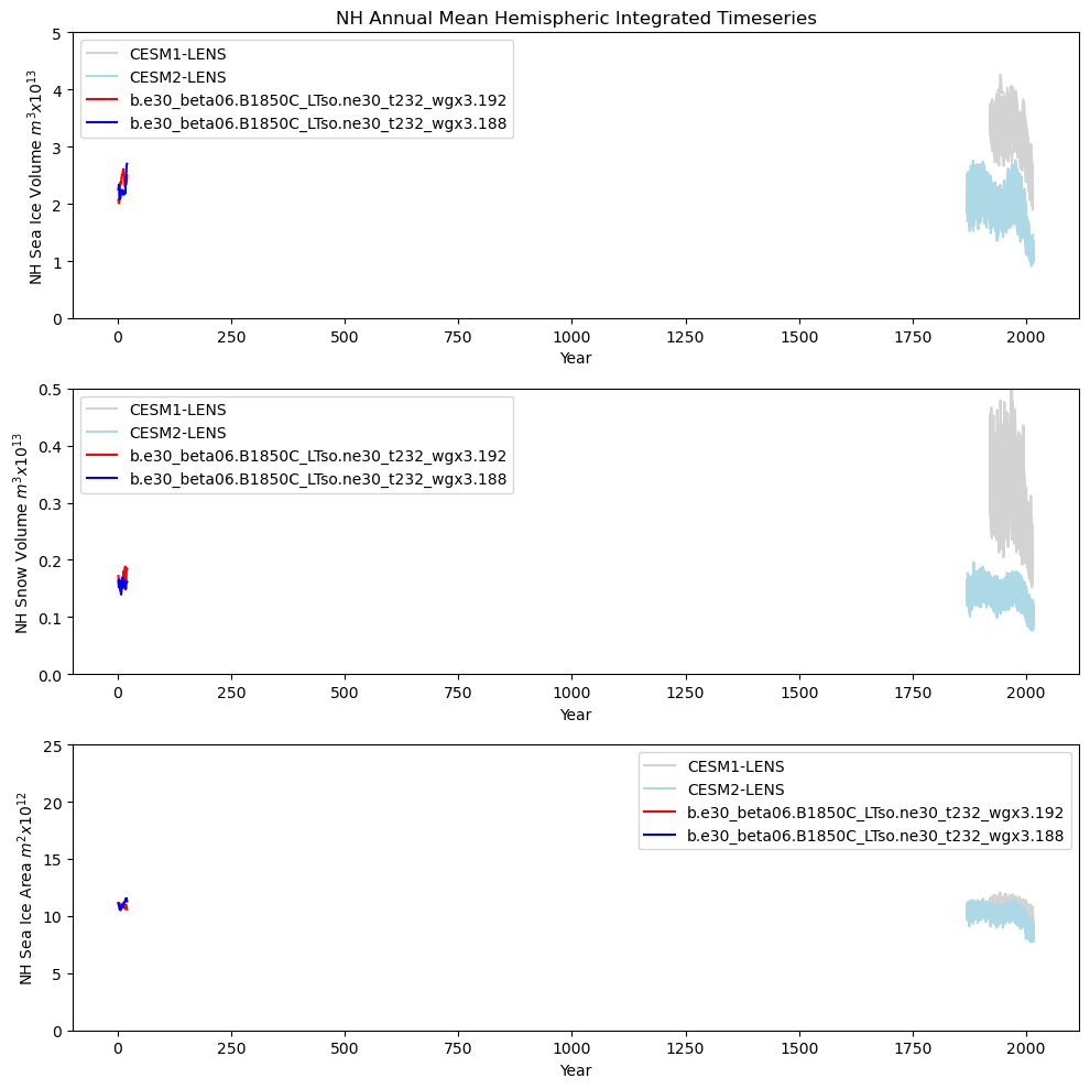
# Northern hemisphere timeseries plot
tag = "NH"

ds1_area_ann = (tarea * ds1_ann["aice"]).where(TLAT > 0).sum(dim=["nj", "ni"]) * 1.0e-12
ds2_area_ann = (tarea * ds2_ann["aice"]).where(TLAT > 0).sum(dim=["nj", "ni"]) * 1.0e-12

ds1_vhi_ann = (tarea * ds1_ann["hi"]).where(TLAT > 0).sum(dim=["nj", "ni"]) * 1.0e-13
ds2_vhi_ann = (tarea * ds2_ann["hi"]).where(TLAT > 0).sum(dim=["nj", "ni"]) * 1.0e-13

ds1_vhs_ann = (tarea * ds1_ann["hs"]).where(TLAT > 0).sum(dim=["nj", "ni"]) * 1.0e-13
ds2_vhs_ann = (tarea * ds2_ann["hs"]).where(TLAT > 0).sum(dim=["nj", "ni"]) * 1.0e-13

# Set up axes
if first_year > 1 and base_first_year > 1:
    model_start_year1 = end_year - len(ds1_area_ann.time) + 1
    model_end_year1 = end_year
    model_start_year2 = base_end_year - len(ds2_area_ann.time) + 1
    model_end_year2 = base_end_year
else:
    model_start_year1 = 1
    model_end_year1 = len(ds1_area_ann.time) + 1
    model_start_year2 = 1
    model_end_year2 = len(ds2_area_ann.time) + 1

x1 = np.linspace(model_start_year1, model_end_year1, len(ds1_area_ann.time))
x2 = np.linspace(model_start_year2, model_end_year2, len(ds2_area_ann.time))

fig = plt.figure(figsize=(10, 10), tight_layout=True)

ax = fig.add_subplot(3, 1, 1)
for i in range(0, 38):
    plt.plot(
        cesm1_years[0:95],
        cesm1_hitot_nh_ann[i, 0:95] * 1.0e-13,
        color="lightgrey",
    )
for i in range(0, 49):
    plt.plot(
        cesm2_years[0:145], cesm2_hitot_nh_ann[i, 0:145] * 1.0e-13, color="lightblue"
    )
plt_plot_len_x_might_be_one(ds1_vhi_ann, x1, x2, color="red")
plt_plot_len_x_might_be_one(ds2_vhi_ann, x2, x1, color="blue")

plt.title(tag + " Annual Mean Hemispheric Integrated Timeseries")
plt.ylim((0, 5))
plt.xlabel("Year")
plt.ylabel(tag + " Sea Ice Volume $m^{3} x 10^{13}$")
plt.legend(handles=[p1, p2, p3, p4])

ax = fig.add_subplot(3, 1, 2)
for i in range(0, 38):
    plt.plot(
        cesm1_years[0:95],
        cesm1_hstot_nh_ann[i, 0:95] * 1.0e-13,
        color="lightgrey",
    )
for i in range(0, 49):
    plt.plot(
        cesm2_years[0:145], cesm2_hstot_nh_ann[i, 0:145] * 1.0e-13, color="lightblue"
    )
plt_plot_len_x_might_be_one(ds1_vhs_ann, x1, x2, color="red")
plt_plot_len_x_might_be_one(ds2_vhs_ann, x2, x1, color="blue")

plt.ylim((0, 0.5))
plt.xlabel("Year")
plt.ylabel(tag + " Snow Volume $m^{3} x 10^{13}$")
plt.legend(handles=[p1, p2, p3, p4])

ax = fig.add_subplot(3, 1, 3)
for i in range(0, 38):
    plt.plot(
        cesm1_years[0:95],
        cesm1_aicetot_nh_ann[i, 0:95] * 1.0e-12,
        color="lightgrey",
    )
for i in range(0, 49):
    plt.plot(
        cesm2_years[0:145], cesm2_aicetot_nh_ann[i, 0:145] * 1.0e-12, color="lightblue"
    )

plt_plot_len_x_might_be_one(ds1_area_ann, x1, x2, color="red")
plt_plot_len_x_might_be_one(ds2_area_ann, x2, x1, color="blue")

plt.ylim((0, 25))
plt.xlabel("Year")
plt.ylabel(tag + " Sea Ice Area $m^{2} x 10^{12}$")
plt.legend(handles=[p1, p2, p3, p4])
<matplotlib.legend.Legend at 0x7f76e82458d0>
Show code cell source
Hide code cell source
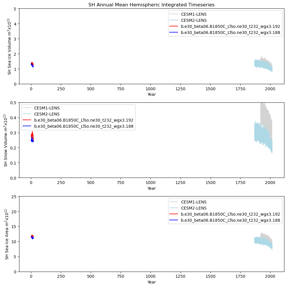
# Southern hemisphere timeseries plot
tag = "SH"

ds1_area_ann = (tarea * ds1_ann["aice"]).where(TLAT < 0).sum(dim=["nj", "ni"]) * 1.0e-12
ds2_area_ann = (tarea * ds2_ann["aice"]).where(TLAT < 0).sum(dim=["nj", "ni"]) * 1.0e-12

ds1_vhi_ann = (tarea * ds1_ann["hi"]).where(TLAT < 0).sum(dim=["nj", "ni"]) * 1.0e-13
ds2_vhi_ann = (tarea * ds2_ann["hi"]).where(TLAT < 0).sum(dim=["nj", "ni"]) * 1.0e-13

ds1_vhs_ann = (tarea * ds1_ann["hs"]).where(TLAT < 0).sum(dim=["nj", "ni"]) * 1.0e-13
ds2_vhs_ann = (tarea * ds2_ann["hs"]).where(TLAT < 0).sum(dim=["nj", "ni"]) * 1.0e-13

fig = plt.figure(figsize=(10, 10), tight_layout=True)

ax = fig.add_subplot(3, 1, 1)
for i in range(0, 38):
    plt.plot(
        cesm1_years[0:95],
        cesm1_hitot_sh_ann[i, 0:95] * 1.0e-13,
        color="lightgrey",
    )
for i in range(0, 49):
    plt.plot(
        cesm2_years[0:145], cesm2_hitot_sh_ann[i, 0:145] * 1.0e-13, color="lightblue"
    )
plt_plot_len_x_might_be_one(ds1_vhi_ann, x1, x2, color="red")
plt_plot_len_x_might_be_one(ds2_vhi_ann, x2, x1, color="blue")

plt.title(tag + " Annual Mean Hemispheric Integrated Timeseries")
plt.ylim((0, 5))
plt.xlabel("Year")
plt.ylabel(tag + " Sea Ice Volume $m^{3} x 10^{13}$")
plt.legend(handles=[p1, p2, p3, p4])

ax = fig.add_subplot(3, 1, 2)
for i in range(0, 38):
    plt.plot(
        cesm1_years[0:95],
        cesm1_hstot_sh_ann[i, 0:95] * 1.0e-13,
        color="lightgrey",
    )
for i in range(0, 49):
    plt.plot(
        cesm2_years[0:145], cesm2_hstot_sh_ann[i, 0:145] * 1.0e-13, color="lightblue"
    )
plt_plot_len_x_might_be_one(ds1_vhs_ann, x1, x2, color="red")
plt_plot_len_x_might_be_one(ds2_vhs_ann, x2, x1, color="blue")

plt.ylim((0, 0.5))
plt.xlabel("Year")
plt.ylabel(tag + " Snow Volume $m^{3} x 10^{13}$")
plt.legend(handles=[p1, p2, p3, p4])

ax = fig.add_subplot(3, 1, 3)
for i in range(0, 38):
    plt.plot(
        cesm1_years[0:95],
        cesm1_aicetot_sh_ann[i, 0:95] * 1.0e-12,
        color="lightgrey",
    )
for i in range(0, 49):
    plt.plot(
        cesm2_years[0:145], cesm2_aicetot_sh_ann[i, 0:145] * 1.0e-12, color="lightblue"
    )
plt_plot_len_x_might_be_one(ds1_area_ann, x1, x2, color="red")
plt_plot_len_x_might_be_one(ds2_area_ann, x2, x1, color="blue")

plt.ylim((0, 25))
plt.xlabel("Year")
plt.ylabel(tag + " Sea Ice Area $m^{2} x 10^{12}$")
plt.legend(handles=[p1, p2, p3, p4])
<matplotlib.legend.Legend at 0x7f76e87994d0>
Annual cycle plots - Ice Area#
Show code cell source
Hide code cell source
# get monthly means from test data
aice1_month = (
    ds1["aice"]
    .isel(time=slice(-climo_nyears1 * 12, None))
    .groupby("time.month")
    .mean(dim="time", skipna=True)
)
aice2_month = (
    ds2["aice"]
    .isel(time=slice(-climo_nyears2 * 12, None))
    .groupby("time.month")
    .mean(dim="time", skipna=True)
)
Show code cell source
Hide code cell source
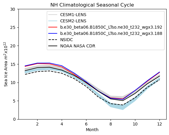
# Northern hemisphere annual cycle plot
tag = "NH"

mask_tmp1_nh = np.where(np.logical_and(aice1_month > 0.15, ds1["TLAT"] > 0), 1.0, 0.0)
mask_tmp2_nh = np.where(np.logical_and(aice2_month > 0.15, ds1["TLAT"] > 0), 1.0, 0.0)

mask_nh_tmp = np.where(ds1["TLAT"] > 0, tarea, 0.0)
mask_nh = xr.DataArray(data=mask_nh_tmp, dims=["nj", "ni"])

area1 = (aice1_month * mask_nh).sum(["ni", "nj"]) * 1.0e-12
area2 = (aice2_month * mask_nh).sum(["ni", "nj"]) * 1.0e-12

months = np.linspace(1, 12, 12)

for i in range(0, 38):
    plt.plot(months, cesm1_aicetot_nh_month[i, :] * 1.0e-12, color="lightgrey")
for i in range(0, 49):
    plt.plot(months, cesm2_aicetot_nh_month[i, :] * 1.0e-12, color="lightblue")
plt.plot(months, area1, color="red")
plt.plot(months, area2, color="blue")
plt.plot(months, nsidc_clim_nh_area, color="black", linestyle="dashed")
plt.plot(months, cdr_nh_clim, color="black")

plt.title(tag + " Climatological Seasonal Cycle")
plt.ylim((0, 30))
plt.xlabel("Month")
plt.ylabel("Sea Ice Area $m^{2} x 10^{12}$")
plt.legend(handles=[p1, p2, p3, p4, p5, p6])
<matplotlib.legend.Legend at 0x7f76e80e71d0>
Show code cell source
Hide code cell source
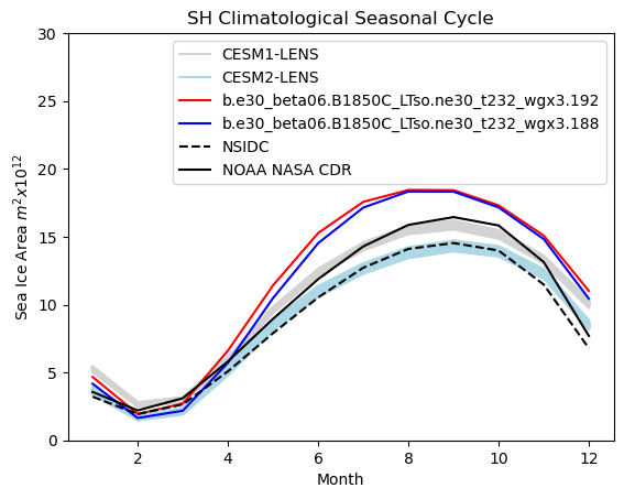
# Southern hemisphere annual cycle plot
tag = "SH"

mask_tmp1_sh = np.where(np.logical_and(aice1_month > 0.15, ds1["TLAT"] < 0), 1.0, 0.0)
mask_tmp2_sh = np.where(np.logical_and(aice2_month > 0.15, ds1["TLAT"] < 0), 1.0, 0.0)

mask_sh_tmp = np.where(ds1["TLAT"] < 0, tarea, 0.0)
mask_sh = xr.DataArray(data=mask_sh_tmp, dims=["nj", "ni"])

area1 = (aice1_month * mask_sh).sum(["ni", "nj"]) * 1.0e-12
area2 = (aice2_month * mask_sh).sum(["ni", "nj"]) * 1.0e-12

for i in range(0, 38):
    plt.plot(months, cesm1_aicetot_sh_month[i, :] * 1.0e-12, color="lightgrey")
for i in range(0, 49):
    plt.plot(months, cesm2_aicetot_sh_month[i, :] * 1.0e-12, color="lightblue")
plt.plot(months, area1, color="red")
plt.plot(months, area2, color="blue")
plt.plot(months, nsidc_clim_sh_area, color="black", linestyle="dashed")
plt.plot(months, cdr_sh_clim, color="black")

plt.title(tag + " Climatological Seasonal Cycle")
plt.ylim((0, 30))
plt.xlabel("Month")
plt.ylabel("Sea Ice Area $m^{2} x 10^{12}$")
plt.legend(handles=[p1, p2, p3, p4, p5, p6])
<matplotlib.legend.Legend at 0x7f76cba7c810>
Annual cycle plots - Ice Volume#
Show code cell source
Hide code cell source
# get monthly means from test data
hi1_month = (
    ds1["hi"]
    .isel(time=slice(-climo_nyears1 * 12, None))
    .groupby("time.month")
    .mean(dim="time", skipna=True)
)
hi2_month = (
    ds2["hi"]
    .isel(time=slice(-climo_nyears2 * 12, None))
    .groupby("time.month")
    .mean(dim="time", skipna=True)
)
Show code cell source
Hide code cell source
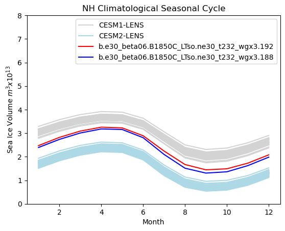
# Northern hemisphere annual cycle plot
tag = "NH"

mask_tmp1_nh = np.where(np.logical_and(hi1_month > 0, ds1["TLAT"] > 0), 1.0, 0.0)
mask_tmp2_nh = np.where(np.logical_and(hi2_month > 0, ds1["TLAT"] > 0), 1.0, 0.0)

mask_nh_tmp = np.where(ds1["TLAT"] > 0, tarea, 0.0)
mask_nh = xr.DataArray(data=mask_nh_tmp, dims=["nj", "ni"])

vol1 = (hi1_month * mask_nh).sum(["ni", "nj"]) * 1.0e-13
vol2 = (hi2_month * mask_nh).sum(["ni", "nj"]) * 1.0e-13

months = np.linspace(1, 12, 12)

for i in range(0, 38):
    plt.plot(months, cesm1_hitot_nh_month[i, :] * 1.0e-13, color="lightgrey")
for i in range(0, 49):
    plt.plot(months, cesm2_hitot_nh_month[i, :] * 1.0e-13, color="lightblue")
plt.plot(months, vol1, color="red")
plt.plot(months, vol2, color="blue")

plt.title(tag + " Climatological Seasonal Cycle")
plt.ylim((0, 8))
plt.xlabel("Month")
plt.ylabel("Sea Ice Volume $m^{3} x 10^{13}$")
plt.legend(handles=[p1, p2, p3, p4])
<matplotlib.legend.Legend at 0x7f76c82b14d0>
Show code cell source
Hide code cell source
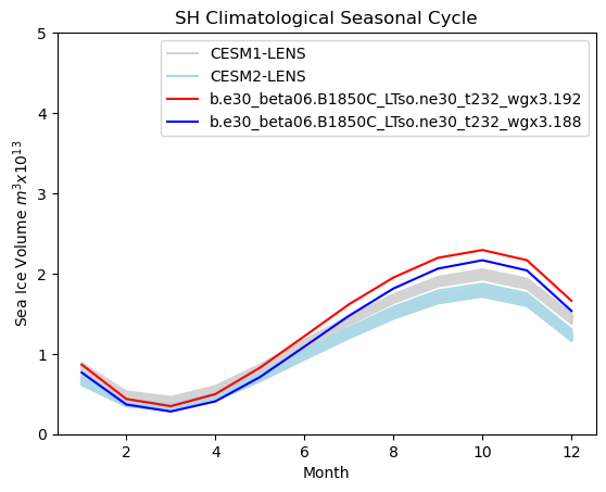
# Southern hemisphere annual cycle plot
tag = "SH"

mask_tmp1_sh = np.where(np.logical_and(hi1_month > 0, ds1["TLAT"] < 0), 1.0, 0.0)
mask_tmp2_sh = np.where(np.logical_and(hi2_month > 0, ds1["TLAT"] < 0), 1.0, 0.0)

mask_sh_tmp = np.where(ds1["TLAT"] < 0, tarea, 0.0)
mask_sh = xr.DataArray(data=mask_sh_tmp, dims=["nj", "ni"])

vol1 = (hi1_month * mask_sh).sum(["ni", "nj"]) * 1.0e-13
vol2 = (hi2_month * mask_sh).sum(["ni", "nj"]) * 1.0e-13

months = np.linspace(1, 12, 12)

for i in range(0, 38):
    plt.plot(months, cesm1_hitot_sh_month[i, :] * 1.0e-13, color="lightgrey")
for i in range(0, 49):
    plt.plot(months, cesm2_hitot_sh_month[i, :] * 1.0e-13, color="lightblue")
plt.plot(months, vol1, color="red")
plt.plot(months, vol2, color="blue")

plt.title(tag + " Climatological Seasonal Cycle")
plt.ylim((0, 5))
plt.xlabel("Month")
plt.ylabel("Sea Ice Volume $m^{3} x 10^{13}$")
plt.legend(handles=[p1, p2, p3, p4])
<matplotlib.legend.Legend at 0x7f76cb721410>
Annual cycle plots - Snow volume#
Show code cell source
Hide code cell source
# get monthly means from test data
hs1_month = (
    ds1["hs"]
    .isel(time=slice(-climo_nyears1 * 12, None))
    .groupby("time.month")
    .mean(dim="time", skipna=True)
)
hs2_month = (
    ds2["hs"]
    .isel(time=slice(-climo_nyears2 * 12, None))
    .groupby("time.month")
    .mean(dim="time", skipna=True)
)
Show code cell source
Hide code cell source
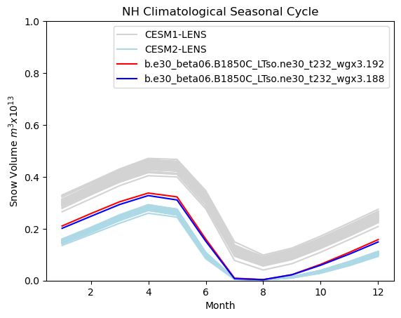
# Northern hemisphere annual cycle plot
tag = "NH"

mask_tmp1_nh = np.where(np.logical_and(hs1_month > 0, ds1["TLAT"] > 0), 1.0, 0.0)
mask_tmp2_nh = np.where(np.logical_and(hs2_month > 0, ds1["TLAT"] > 0), 1.0, 0.0)

mask_nh_tmp = np.where(ds1["TLAT"] > 0, tarea, 0.0)
mask_nh = xr.DataArray(data=mask_nh_tmp, dims=["nj", "ni"])

vol1 = (hs1_month * mask_nh).sum(["ni", "nj"]) * 1.0e-13
vol2 = (hs2_month * mask_nh).sum(["ni", "nj"]) * 1.0e-13

months = np.linspace(1, 12, 12)

for i in range(0, 38):
    plt.plot(months, cesm1_hstot_nh_month[i, :] * 1.0e-13, color="lightgrey")
for i in range(0, 49):
    plt.plot(months, cesm2_hstot_nh_month[i, :] * 1.0e-13, color="lightblue")
plt.plot(months, vol1, color="red")
plt.plot(months, vol2, color="blue")

plt.title(tag + " Climatological Seasonal Cycle")
plt.ylim((0, 1))
plt.xlabel("Month")
plt.ylabel("Snow Volume $m^{3} x 10^{13}$")
plt.legend(handles=[p1, p2, p3, p4])
<matplotlib.legend.Legend at 0x7f76cb07b950>
Show code cell source
Hide code cell source
# Southern hemisphere annual cycle plot
tag = "SH"

mask_tmp1_sh = np.where(np.logical_and(hs1_month > 0, ds1["TLAT"] < 0), 1.0, 0.0)
mask_tmp2_sh = np.where(np.logical_and(hs2_month > 0, ds1["TLAT"] < 0), 1.0, 0.0)

mask_sh_tmp = np.where(ds1["TLAT"] < 0, tarea, 0.0)
mask_sh = xr.DataArray(data=mask_sh_tmp, dims=["nj", "ni"])

vol1 = (hs1_month * mask_sh).sum(["ni", "nj"]) * 1.0e-13
vol2 = (hs2_month * mask_sh).sum(["ni", "nj"]) * 1.0e-13

months = np.linspace(1, 12, 12)

for i in range(0, 38):
    plt.plot(months, cesm1_hstot_sh_month[i, :] * 1.0e-13, color="lightgrey")
for i in range(0, 49):
    plt.plot(months, cesm2_hstot_sh_month[i, :] * 1.0e-13, color="lightblue")
plt.plot(months, vol1, color="red")
plt.plot(months, vol2, color="blue")

plt.title(tag + " Climatological Seasonal Cycle")
plt.ylim((0, 1))
plt.xlabel("Month")
plt.ylabel("Snow Volume $m^{3} x 10^{13}$")
plt.legend(handles=[p1, p2, p3, p4])
<matplotlib.legend.Legend at 0x7f76caec9710>

Monthly Analysis for Minimum and Maximum Months#
NH#
Maximum - March
Minimum - September
Ice Area#
Show code cell source
Hide code cell source
ds1_area = (tarea * ds1.aice).isel(time=slice(-climo_nyears1 * 12, None)).where(
    TLAT > 0
).sum(dim=["nj", "ni"]) * 1.0e-12
ds2_area = (tarea * ds2.aice).isel(time=slice(-climo_nyears2 * 12, None)).where(
    TLAT > 0
).sum(dim=["nj", "ni"]) * 1.0e-12
Execution using papermill encountered an exception here and stopped:
Show code cell source
Hide code cell source
tag = "NH"

ds1_mar_nh = ds1_area.sel(time=(ds1_area.time.dt.month == 3))
ds2_mar_nh = ds2_area.sel(time=(ds2_area.time.dt.month == 3))

cesm1_aicetot_nh_mar = ds_cesm1_aicetot_nh["aice_monthly"].isel(nmonth=2)
cesm2_aicetot_nh_mar = ds_cesm2_aicetot_nh["aice_monthly"].isel(nmonth=2)

cesm1_aicetot_sh_sep = ds_cesm1_aicetot_sh["aice_monthly"].isel(nmonth=8)
cesm2_aicetot_sh_sep = ds_cesm2_aicetot_sh["aice_monthly"].isel(nmonth=8)

# Set up axes
if first_year > 1 and base_first_year > 1:
    model_start_year1 = end_year - len(ds1_mar_nh.time) + 1
    model_end_year1 = end_year
    model_start_year2 = base_end_year - len(ds2_mar_nh.time) + 1
    model_end_year2 = base_end_year
    lens1_start_year = ds_cesm1_aicetot_nh.year[60]
    lens1_end_year = ds_cesm1_aicetot_nh.year[95]
    lens2_start_year = ds_cesm2_aicetot_nh.year[110]
    lens2_end_year = ds_cesm2_aicetot_nh.year[145]
else:
    model_start_year1 = 1
    model_end_year1 = len(ds1_mar_nh.time) + 1
    model_start_year2 = 1
    model_end_year2 = len(ds2_mar_nh.time) + 1
    lens1_start_year = 1
    lens1_end_year = 36
    lens2_start_year = 1
    lens2_end_year = 36

del x1
del x2

x1 = np.linspace(model_start_year1, model_end_year1, len(ds1_mar_nh.time))
x2 = np.linspace(model_start_year2, model_end_year2, len(ds2_mar_nh.time))
x3 = np.linspace(lens1_start_year, lens1_end_year, 36)
x4 = np.linspace(lens2_start_year, lens2_end_year, 36)

obs_first_year = 0
if first_year > 1 and base_first_year > 1:
    obs_first_year = 1979
x5 = np.linspace(1, 36, 36) + obs_first_year
x6 = np.linspace(1, 45, 45) + obs_first_year

# Make Plot - two subplots - note it's nrow x ncol x index (starting upper left)
fig = plt.figure(figsize=(20, 7))

# First panel, timeseries
ax = fig.add_subplot(1, 2, 1)
for i in range(0, 38):
    ax.plot(
        x3,
        cesm1_aicetot_nh_mar.isel(n_members=i, nyr=slice(60, 96)) * 1.0e-12,
        color="lightgrey",
    )
for i in range(0, 49):
    ax.plot(
        x4,
        cesm2_aicetot_nh_mar.isel(n_members=i, nyr=slice(110, 146)) * 1.0e-12,
        color="lightblue",
    )
plt_plot_len_x_might_be_one(ds1_mar_nh, x1, x2, color="red")
plt_plot_len_x_might_be_one(ds2_mar_nh, x2, x1, color="blue")
ax.plot(x5, mar_area_nh[0:36], color="black", linestyle="dashed")
ax.plot(x6, cdr_nh_mar, color="black")

plt.title(tag + " March Mean Sea Ice Area")
plt.ylim((5, 25))
plt.xlabel("Year")
plt.ylabel("Sea Ice Area $m^{2}x10^{12}$")
plt.legend(handles=[p1, p2, p3, p4, p5, p6])

### Second panel, boxplot
ax = fig.add_subplot(1, 2, 2)
# get just last years of large ensembles and one dimensionalize them
cesm1_tmp = (
    cesm1_aicetot_nh_mar.isel(nyr=slice(60, 96)).stack(new=("n_members", "nyr"))
    * 1.0e-12
)
cesm2_tmp = (
    cesm2_aicetot_nh_mar.isel(nyr=slice(110, 146)).stack(new=("n_members", "nyr"))
    * 1.0e-12
)

# plot boxes
boxplots1 = ax.boxplot(ds1_mar_nh, showfliers=False, autorange=False, positions=[0.25])
boxplots2 = ax.boxplot(ds2_mar_nh, showfliers=False, autorange=False, positions=[0.5])
boxplots3 = ax.boxplot(
    mar_area_nh[-35::], showfliers=False, autorange=False, positions=[0.75]
)
boxplots35 = ax.boxplot(cdr_nh_mar, showfliers=False, autorange=False, positions=[1.0])
boxplots4 = ax.boxplot(cesm1_tmp, showfliers=False, autorange=False, positions=[1.25])
boxplots5 = ax.boxplot(cesm2_tmp, showfliers=False, autorange=False, positions=[1.5])

# set colors for each box
setBoxColor(boxplots1, 8 * ["red"])
setBoxColor(boxplots2, 8 * ["blue"])
setBoxColor(boxplots3, 8 * ["black"])
setBoxColor(boxplots35, 8 * ["black"])
setBoxColor(boxplots4, 8 * ["lightgrey"])
setBoxColor(boxplots5, 8 * ["lightblue"])

# set plot details
plt.title(tag + " March Mean Sea Ice Area Range")
plt.ylabel("Sea Ice Area $m^{2}x10^{12}$")
plt.ylim((5, 25))
plt.xlim([0, 1.5])
plt.xticks(visible=False)
---------------------------------------------------------------------------
ValueError                                Traceback (most recent call last)
Cell In[26], line 37
     35 x1 = np.linspace(model_start_year1, model_end_year1, len(ds1_mar_nh.time))
     36 x2 = np.linspace(model_start_year2, model_end_year2, len(ds2_mar_nh.time))
---> 37 x3 = np.linspace(lens1_start_year, lens1_end_year, 36)
     38 x4 = np.linspace(lens2_start_year, lens2_end_year, 36)
     40 obs_first_year = 0

File /glade/work/hannay/miniconda3/envs/cupid-analysis/lib/python3.11/site-packages/numpy/_core/function_base.py:183, in linspace(start, stop, num, endpoint, retstep, dtype, axis, device)
    180 if integer_dtype:
    181     _nx.floor(y, out=y)
--> 183 y = conv.wrap(y.astype(dtype, copy=False))
    184 if retstep:
    185     return y, step

File /glade/work/hannay/miniconda3/envs/cupid-analysis/lib/python3.11/site-packages/xarray/core/dataarray.py:4808, in DataArray.__array_wrap__(self, obj, context, return_scalar)
   4807 def __array_wrap__(self, obj, context=None, return_scalar=False) -> Self:
-> 4808     new_var = self.variable.__array_wrap__(obj, context, return_scalar)
   4809     return self._replace(new_var)

File /glade/work/hannay/miniconda3/envs/cupid-analysis/lib/python3.11/site-packages/xarray/core/variable.py:2316, in Variable.__array_wrap__(self, obj, context, return_scalar)
   2315 def __array_wrap__(self, obj, context=None, return_scalar=False):
-> 2316     return Variable(self.dims, obj)

File /glade/work/hannay/miniconda3/envs/cupid-analysis/lib/python3.11/site-packages/xarray/core/variable.py:365, in Variable.__init__(self, dims, data, attrs, encoding, fastpath)
    337 def __init__(
    338     self,
    339     dims,
   (...)    343     fastpath=False,
    344 ):
    345     """
    346     Parameters
    347     ----------
   (...)    363         unrecognized encoding items.
    364     """
--> 365     super().__init__(
    366         dims=dims, data=as_compatible_data(data, fastpath=fastpath), attrs=attrs
    367     )
    369     self._encoding = None
    370     if encoding is not None:

File /glade/work/hannay/miniconda3/envs/cupid-analysis/lib/python3.11/site-packages/xarray/namedarray/core.py:264, in NamedArray.__init__(self, dims, data, attrs)
    257 def __init__(
    258     self,
    259     dims: _DimsLike,
    260     data: duckarray[Any, _DType_co],
    261     attrs: _AttrsLike = None,
    262 ):
    263     self._data = data
--> 264     self._dims = self._parse_dimensions(dims)
    265     self._attrs = dict(attrs) if attrs else None

File /glade/work/hannay/miniconda3/envs/cupid-analysis/lib/python3.11/site-packages/xarray/namedarray/core.py:508, in NamedArray._parse_dimensions(self, dims)
    506 dims = (dims,) if isinstance(dims, str) else tuple(dims)
    507 if len(dims) != self.ndim:
--> 508     raise ValueError(
    509         f"dimensions {dims} must have the same length as the "
    510         f"number of data dimensions, ndim={self.ndim}"
    511     )
    512 if len(set(dims)) < len(dims):
    513     repeated_dims = {d for d in dims if dims.count(d) > 1}

ValueError: dimensions () must have the same length as the number of data dimensions, ndim=1
Show code cell source
Hide code cell source
tag = "NH"

ds1_sep_nh = ds1_area.sel(time=(ds1_area.time.dt.month == 9))
ds2_sep_nh = ds2_area.sel(time=(ds2_area.time.dt.month == 9))

cesm1_aicetot_nh_sep = ds_cesm1_aicetot_nh["aice_monthly"].isel(nmonth=8)
cesm2_aicetot_nh_sep = ds_cesm2_aicetot_nh["aice_monthly"].isel(nmonth=8)

# Make Plot - two subplots - note it's nrow x ncol x index (starting upper left)
fig = plt.figure(figsize=(20, 7))

### First panel, timeseries
ax = fig.add_subplot(1, 2, 1)
for i in range(0, 38):
    ax.plot(
        x3,
        cesm1_aicetot_nh_sep.isel(n_members=i, nyr=slice(60, 96)) * 1.0e-12,
        color="lightgrey",
    )
for i in range(0, 49):
    ax.plot(
        x4,
        cesm2_aicetot_nh_sep.isel(n_members=i, nyr=slice(110, 146)) * 1.0e-12,
        color="lightblue",
    )
plt_plot_len_x_might_be_one(ds1_sep_nh, x1, x2, color="red")
plt_plot_len_x_might_be_one(ds2_sep_nh, x2, x1, color="blue")
ax.plot(x5, sep_area_nh[0:36], color="black", linestyle="dashed")
ax.plot(x6, cdr_nh_sep, color="black")

plt.title(tag + " September Mean Sea Ice Area")
plt.ylim((0, 15))
plt.xlabel("Year")
plt.ylabel("Sea Ice Area $m^{2}x10^{12}$")
plt.legend(handles=[p1, p2, p3, p4, p5, p6])

### Second panel, boxplot
ax = fig.add_subplot(1, 2, 2)
# get just last years of large ensembles and one dimensionalize them
cesm1_tmp = (
    cesm1_aicetot_nh_sep.isel(nyr=slice(60, 96)).stack(new=("n_members", "nyr"))
    * 1.0e-12
)
cesm2_tmp = (
    cesm2_aicetot_nh_sep.isel(nyr=slice(110, 146)).stack(new=("n_members", "nyr"))
    * 1.0e-12
)

# plot boxes
boxplots1 = ax.boxplot(ds1_sep_nh, showfliers=False, autorange=False, positions=[0.25])
boxplots2 = ax.boxplot(ds2_sep_nh, showfliers=False, autorange=False, positions=[0.5])
boxplots3 = ax.boxplot(
    sep_area_nh[-35::], showfliers=False, autorange=False, positions=[0.75]
)
boxplots35 = ax.boxplot(cdr_nh_sep, showfliers=False, autorange=False, positions=[1.0])
boxplots4 = ax.boxplot(cesm1_tmp, showfliers=False, autorange=False, positions=[1.25])
boxplots5 = ax.boxplot(cesm2_tmp, showfliers=False, autorange=False, positions=[1.5])

# set colors for each box
setBoxColor(boxplots1, 8 * ["red"])
setBoxColor(boxplots2, 8 * ["blue"])
setBoxColor(boxplots3, 8 * ["black"])
setBoxColor(boxplots35, 8 * ["black"])
setBoxColor(boxplots4, 8 * ["lightgrey"])
setBoxColor(boxplots5, 8 * ["lightblue"])

# set plot details
plt.title(tag + " September Mean Sea Ice Area Range")
plt.ylabel("Sea Ice Area $m^{2}x10^{12}$")
plt.ylim((0, 15))
plt.xlim([0, 1.5])
plt.xticks(visible=False)
Ice Volume#
Show code cell source
Hide code cell source
ds1_vol = (tarea * ds1.hi).isel(time=slice(-climo_nyears1 * 12, None)).where(
    TLAT > 0
).sum(dim=["nj", "ni"]) * 1.0e-13
ds2_vol = (tarea * ds2.hi).isel(time=slice(-climo_nyears2 * 12, None)).where(
    TLAT > 0
).sum(dim=["nj", "ni"]) * 1.0e-13
Show code cell source
Hide code cell source
tag = "NH"

ds1_mar_nh = ds1_vol.sel(time=(ds1_vol.time.dt.month == 3))
ds2_mar_nh = ds2_vol.sel(time=(ds2_vol.time.dt.month == 3))

cesm1_hitot_nh_mar = ds_cesm1_hitot_nh["hi_monthly"].isel(nmonth=2)
cesm2_hitot_nh_mar = ds_cesm2_hitot_nh["hi_monthly"].isel(nmonth=2)

# Make Plot - two subplots - note it's nrow x ncol x index (starting upper left)
fig = plt.figure(figsize=(20, 7))

### First panel, timeseries
ax = fig.add_subplot(1, 2, 1)
for i in range(0, 38):
    ax.plot(
        x3,
        cesm1_hitot_nh_mar.isel(n_members=i, nyr=slice(60, 96)) * 1.0e-13,
        color="lightgrey",
    )
for i in range(0, 49):
    ax.plot(
        x4,
        cesm2_hitot_nh_mar.isel(n_members=i, nyr=slice(110, 146)) * 1.0e-13,
        color="lightblue",
    )
plt_plot_len_x_might_be_one(ds1_mar_nh, x1, x2, color="red")
plt_plot_len_x_might_be_one(ds2_mar_nh, x2, x1, color="blue")

plt.title(tag + " March Mean Sea Ice Volume")
plt.ylim((0, 10))
plt.xlabel("Year")
plt.ylabel("Sea Ice Volume $m^{3}x10^{13}$")
plt.legend(handles=[p1, p2, p3, p4])

### Second panel, boxplot
ax = fig.add_subplot(1, 2, 2)
# get just last years of large ensembles and one dimensionalize them
cesm1_tmp = (
    cesm1_hitot_nh_mar.isel(nyr=slice(60, 96)).stack(new=("n_members", "nyr")) * 1.0e-13
)
cesm2_tmp = (
    cesm2_hitot_nh_mar.isel(nyr=slice(110, 146)).stack(new=("n_members", "nyr"))
    * 1.0e-13
)

# plot boxes
boxplots1 = ax.boxplot(ds1_mar_nh, showfliers=False, autorange=False, positions=[0.25])
boxplots2 = ax.boxplot(ds2_mar_nh, showfliers=False, autorange=False, positions=[0.5])
boxplots4 = ax.boxplot(cesm1_tmp, showfliers=False, autorange=False, positions=[1.0])
boxplots5 = ax.boxplot(cesm2_tmp, showfliers=False, autorange=False, positions=[1.25])

# set colors for each box
setBoxColor(boxplots1, 8 * ["red"])
setBoxColor(boxplots2, 8 * ["blue"])
setBoxColor(boxplots4, 8 * ["lightgrey"])
setBoxColor(boxplots5, 8 * ["lightblue"])

# set plot details
plt.title(tag + " March Mean Sea Ice Volume Range")
plt.ylabel("Sea Ice Area $m^{3}x10^{13}$")
plt.ylim((0, 10))
plt.xlim([0, 1.5])
plt.xticks(visible=False)
Show code cell source
Hide code cell source
tag = "NH"

ds1_sep_nh = ds1_vol.sel(time=(ds1_vol.time.dt.month == 9))
ds2_sep_nh = ds2_vol.sel(time=(ds2_vol.time.dt.month == 9))

cesm1_hitot_nh_sep = ds_cesm1_hitot_nh["hi_monthly"].isel(nmonth=8)
cesm2_hitot_nh_sep = ds_cesm2_hitot_nh["hi_monthly"].isel(nmonth=8)

# Make Plot - two subplots - note it's nrow x ncol x index (starting upper left)
fig = plt.figure(figsize=(20, 7))

### First panel, timeseries
ax = fig.add_subplot(1, 2, 1)
for i in range(0, 38):
    ax.plot(
        x3,
        cesm1_hitot_nh_sep.isel(n_members=i, nyr=slice(60, 96)) * 1.0e-13,
        color="lightgrey",
    )
for i in range(0, 49):
    ax.plot(
        x4,
        cesm2_hitot_nh_sep.isel(n_members=i, nyr=slice(110, 146)) * 1.0e-13,
        color="lightblue",
    )
plt_plot_len_x_might_be_one(ds1_sep_nh, x1, x2, color="red")
plt_plot_len_x_might_be_one(ds2_sep_nh, x2, x1, color="blue")

plt.title(tag + " September Mean Sea Ice Volume")
plt.ylim((0, 6))
plt.xlabel("Year")
plt.ylabel("Sea Ice Volume $m^{3}x10^{13}$")
plt.legend(handles=[p1, p2, p3, p4])

### Second panel, boxplot
ax = fig.add_subplot(1, 2, 2)
# get just last years of large ensembles and one dimensionalize them
cesm1_tmp = (
    cesm1_hitot_nh_sep.isel(nyr=slice(60, 96)).stack(new=("n_members", "nyr")) * 1.0e-13
)
cesm2_tmp = (
    cesm2_hitot_nh_sep.isel(nyr=slice(110, 146)).stack(new=("n_members", "nyr"))
    * 1.0e-13
)

# plot boxes
boxplots1 = ax.boxplot(ds1_sep_nh, showfliers=False, autorange=False, positions=[0.25])
boxplots2 = ax.boxplot(ds2_sep_nh, showfliers=False, autorange=False, positions=[0.5])
boxplots4 = ax.boxplot(cesm1_tmp, showfliers=False, autorange=False, positions=[1.0])
boxplots5 = ax.boxplot(cesm2_tmp, showfliers=False, autorange=False, positions=[1.25])

# set colors for each box
setBoxColor(boxplots1, 8 * ["red"])
setBoxColor(boxplots2, 8 * ["blue"])
setBoxColor(boxplots4, 8 * ["lightgrey"])
setBoxColor(boxplots5, 8 * ["lightblue"])

# set plot details
plt.title(tag + " September Mean Sea Ice Volume Range")
plt.ylabel("Sea Ice Area $m^{3}x10^{13}$")
plt.ylim((0, 6))
plt.xlim([0, 1.5])
plt.xticks(visible=False)
SH#
Maximum - September
Minimum - February
Ice Area#
Show code cell source
Hide code cell source
ds1_area = (tarea * ds1.aice).isel(time=slice(-climo_nyears1 * 12, None)).where(
    TLAT < 0
).sum(dim=["nj", "ni"]) * 1.0e-12
ds2_area = (tarea * ds2.aice).isel(time=slice(-climo_nyears2 * 12, None)).where(
    TLAT < 0
).sum(dim=["nj", "ni"]) * 1.0e-12
Show code cell source
Hide code cell source
tag = "SH"

ds1_feb_sh = ds1_area.sel(time=(ds1_area.time.dt.month == 2))
ds2_feb_sh = ds2_area.sel(time=(ds2_area.time.dt.month == 2))

cesm1_aicetot_sh_feb = ds_cesm1_aicetot_sh["aice_monthly"].isel(nmonth=1)
cesm2_aicetot_sh_feb = ds_cesm2_aicetot_sh["aice_monthly"].isel(nmonth=1)

# Make Plot - two subplots - note it's nrow x ncol x index (starting upper left)
fig = plt.figure(figsize=(20, 7))

### First panel, timeseries
ax = fig.add_subplot(1, 2, 1)
for i in range(0, 38):
    ax.plot(
        x3,
        cesm1_aicetot_sh_feb.isel(n_members=i, nyr=slice(60, 96)) * 1.0e-12,
        color="lightgrey",
    )
for i in range(0, 49):
    ax.plot(
        x4,
        cesm2_aicetot_sh_feb.isel(n_members=i, nyr=slice(110, 146)) * 1.0e-12,
        color="lightblue",
    )
plt_plot_len_x_might_be_one(ds1_feb_sh, x1, x2, color="red")
plt_plot_len_x_might_be_one(ds2_feb_sh, x2, x1, color="blue")
ax.plot(x5, feb_area_sh[0:36], color="black")
ax.plot(x6, cdr_sh_feb, color="black")

plt.title(tag + " February Mean Sea Ice Area")
plt.ylim((0, 10))
plt.xlabel("Year")
plt.ylabel("Sea Ice Area $m^{2}x10^{12}$")
plt.legend(handles=[p1, p2, p3, p4, p5, p6])

### Second panel, boxplot
ax = fig.add_subplot(1, 2, 2)
# get just last years of large ensembles and one dimensionalize them
cesm1_tmp = (
    cesm1_aicetot_sh_feb.isel(nyr=slice(60, 96)).stack(new=("n_members", "nyr"))
    * 1.0e-12
)
cesm2_tmp = (
    cesm2_aicetot_sh_feb.isel(nyr=slice(110, 146)).stack(new=("n_members", "nyr"))
    * 1.0e-12
)

# plot boxes
boxplots1 = ax.boxplot(ds1_feb_sh, showfliers=False, autorange=False, positions=[0.25])
boxplots2 = ax.boxplot(ds2_feb_sh, showfliers=False, autorange=False, positions=[0.5])
boxplots3 = ax.boxplot(
    feb_area_sh[-35::], showfliers=False, autorange=False, positions=[0.75]
)
boxplots35 = ax.boxplot(cdr_sh_feb, showfliers=False, autorange=False, positions=[1.0])
boxplots4 = ax.boxplot(cesm1_tmp, showfliers=False, autorange=False, positions=[1.2])
boxplots5 = ax.boxplot(cesm2_tmp, showfliers=False, autorange=False, positions=[1.5])

# set colors for each box
setBoxColor(boxplots1, 8 * ["red"])
setBoxColor(boxplots2, 8 * ["blue"])
setBoxColor(boxplots3, 8 * ["black"])
setBoxColor(boxplots35, 8 * ["black"])
setBoxColor(boxplots4, 8 * ["lightgrey"])
setBoxColor(boxplots5, 8 * ["lightblue"])

# set plot details
plt.title(tag + " February Mean Sea Ice Area Range")
plt.ylabel("Sea Ice Area $m^{2}x10^{12}$")
plt.ylim((0, 10))
plt.xlim([0, 1.5])
plt.xticks(visible=False)
Show code cell source
Hide code cell source
tag = "SH"

ds1_sep_sh = ds1_area.sel(time=(ds1_area.time.dt.month == 9))
ds2_sep_sh = ds2_area.sel(time=(ds2_area.time.dt.month == 9))

cesm1_aicetot_sh_sep = ds_cesm1_aicetot_sh["aice_monthly"].isel(nmonth=8)
cesm2_aicetot_sh_sep = ds_cesm2_aicetot_sh["aice_monthly"].isel(nmonth=8)

# Make Plot - two subplots - note it's nrow x ncol x index (starting upper left)
fig = plt.figure(figsize=(20, 7))

### First panel, timeseries
ax = fig.add_subplot(1, 2, 1)
for i in range(0, 38):
    ax.plot(
        x3,
        cesm1_aicetot_sh_sep.isel(n_members=i, nyr=slice(60, 96)) * 1.0e-12,
        color="lightgrey",
    )
for i in range(0, 49):
    ax.plot(
        x4,
        cesm2_aicetot_sh_sep.isel(n_members=i, nyr=slice(110, 146)) * 1.0e-12,
        color="lightblue",
    )
plt_plot_len_x_might_be_one(ds1_sep_sh, x1, x2, color="red")
plt_plot_len_x_might_be_one(ds2_sep_sh, x2, x1, color="blue")
ax.plot(x5, sep_area_sh[0:36], color="black", linestyle="dashed")
ax.plot(x6, cdr_sh_sep, color="black")

plt.title(tag + " September Mean Sea Ice Area")
plt.ylim((10, 30))
plt.xlabel("Year")
plt.ylabel("Sea Ice Area $m^{2}x10^{12}$")
plt.legend(handles=[p1, p2, p3, p4, p5, p6])

### Second panel, boxplot
ax = fig.add_subplot(1, 2, 2)
# get just last years of large ensembles and one dimensionalize them
cesm1_tmp = (
    cesm1_aicetot_sh_sep.isel(nyr=slice(60, 96)).stack(new=("n_members", "nyr"))
    * 1.0e-12
)
cesm2_tmp = (
    cesm2_aicetot_sh_sep.isel(nyr=slice(110, 146)).stack(new=("n_members", "nyr"))
    * 1.0e-12
)

# plot boxes
boxplots1 = ax.boxplot(ds1_sep_sh, showfliers=False, autorange=False, positions=[0.25])
boxplots2 = ax.boxplot(ds2_sep_sh, showfliers=False, autorange=False, positions=[0.5])
boxplots3 = ax.boxplot(
    sep_area_sh[-35::], showfliers=False, autorange=False, positions=[0.75]
)
boxplots35 = ax.boxplot(cdr_sh_sep, showfliers=False, autorange=False, positions=[1.0])
boxplots4 = ax.boxplot(cesm1_tmp, showfliers=False, autorange=False, positions=[1.25])
boxplots5 = ax.boxplot(cesm2_tmp, showfliers=False, autorange=False, positions=[1.5])

# set colors for each box
setBoxColor(boxplots1, 8 * ["red"])
setBoxColor(boxplots2, 8 * ["blue"])
setBoxColor(boxplots3, 8 * ["black"])
setBoxColor(boxplots35, 8 * ["black"])
setBoxColor(boxplots4, 8 * ["lightgrey"])
setBoxColor(boxplots5, 8 * ["lightblue"])

# set plot details
plt.title(tag + " September Mean Sea Ice Area Range")
plt.ylabel("Sea Ice Area $m^{2}x10^{12}$")
plt.ylim((10, 30))
plt.xlim([0, 1.5])
plt.xticks(visible=False)
Ice Volume#
Show code cell source
Hide code cell source
ds1_vol = (tarea * ds1.hi).isel(time=slice(-climo_nyears1 * 12, None)).where(
    TLAT < 0
).sum(dim=["nj", "ni"]) * 1.0e-13
ds2_vol = (tarea * ds2.hi).isel(time=slice(-climo_nyears2 * 12, None)).where(
    TLAT < 0
).sum(dim=["nj", "ni"]) * 1.0e-13
Show code cell source
Hide code cell source
tag = "SH"

ds1_feb_sh = ds1_vol.sel(time=(ds1_vol.time.dt.month == 3))
ds2_feb_sh = ds2_vol.sel(time=(ds2_vol.time.dt.month == 3))

cesm1_hitot_sh_feb = ds_cesm1_hitot_sh["hi_monthly"].isel(nmonth=2)
cesm2_hitot_sh_feb = ds_cesm2_hitot_sh["hi_monthly"].isel(nmonth=2)

# Make Plot - two subplots - note it's nrow x ncol x index (starting upper left)
fig = plt.figure(figsize=(20, 7))

### First panel, timeseries
ax = fig.add_subplot(1, 2, 1)
for i in range(0, 38):
    ax.plot(
        x3,
        cesm1_hitot_sh_feb.isel(n_members=i, nyr=slice(60, 96)) * 1.0e-13,
        color="lightgrey",
    )
for i in range(0, 49):
    ax.plot(
        x4,
        cesm2_hitot_sh_feb.isel(n_members=i, nyr=slice(110, 146)) * 1.0e-13,
        color="lightblue",
    )
plt_plot_len_x_might_be_one(ds1_feb_sh, x1, x2, color="red")
plt_plot_len_x_might_be_one(ds2_feb_sh, x2, x1, color="blue")

plt.title(tag + " February Mean Sea Ice Volume")
plt.ylim((0, 2))
plt.xlabel("Year")
plt.ylabel("Sea Ice Volume $m^{3}x10^{13}$")
plt.legend(handles=[p1, p2, p3, p4])

### Second panel, boxplot
ax = fig.add_subplot(1, 2, 2)
# get just last years of large ensembles and one dimensionalize them
cesm1_tmp = (
    cesm1_hitot_sh_feb.isel(nyr=slice(60, 96)).stack(new=("n_members", "nyr")) * 1.0e-13
)
cesm2_tmp = (
    cesm2_hitot_sh_feb.isel(nyr=slice(110, 146)).stack(new=("n_members", "nyr"))
    * 1.0e-13
)

# plot boxes
boxplots1 = ax.boxplot(ds1_feb_sh, showfliers=False, autorange=False, positions=[0.25])
boxplots2 = ax.boxplot(ds2_feb_sh, showfliers=False, autorange=False, positions=[0.5])
boxplots4 = ax.boxplot(cesm1_tmp, showfliers=False, autorange=False, positions=[1.0])
boxplots5 = ax.boxplot(cesm2_tmp, showfliers=False, autorange=False, positions=[1.25])

# set colors for each box
setBoxColor(boxplots1, 8 * ["red"])
setBoxColor(boxplots2, 8 * ["blue"])
setBoxColor(boxplots4, 8 * ["lightgrey"])
setBoxColor(boxplots5, 8 * ["lightblue"])

# set plot details
plt.title(tag + " February Mean Sea Ice Volume Range")
plt.ylabel("Sea Ice Area $m^{3}x10^{13}$")
plt.ylim((0, 2))
plt.xlim([0, 1.5])
plt.xticks(visible=False)
Show code cell source
Hide code cell source
tag = "SH"

ds1_sep_sh = ds1_vol.sel(time=(ds1_vol.time.dt.month == 9))
ds2_sep_sh = ds2_vol.sel(time=(ds2_vol.time.dt.month == 9))

cesm1_hitot_sh_sep = ds_cesm1_hitot_sh["hi_monthly"].isel(nmonth=8)
cesm2_hitot_sh_sep = ds_cesm2_hitot_sh["hi_monthly"].isel(nmonth=8)

# Make Plot - two subplots - note it's nrow x ncol x index (starting upper left)
fig = plt.figure(figsize=(20, 7))

### First panel, timeseries
ax = fig.add_subplot(1, 2, 1)
for i in range(0, 38):
    ax.plot(
        x3,
        cesm1_hitot_sh_sep.isel(n_members=i, nyr=slice(60, 96)) * 1.0e-13,
        color="lightgrey",
    )
for i in range(0, 49):
    ax.plot(
        x4,
        cesm2_hitot_sh_sep.isel(n_members=i, nyr=slice(110, 146)) * 1.0e-13,
        color="lightblue",
    )
plt_plot_len_x_might_be_one(ds1_sep_sh, x1, x2, color="red")
plt_plot_len_x_might_be_one(ds2_sep_sh, x2, x1, color="blue")

plt.title(tag + " September Mean Sea Ice Volume")
plt.ylim((0, 6))
plt.xlabel("Year")
plt.ylabel("Sea Ice Volume $m^{3}x10^{13}$")
plt.legend(handles=[p1, p2, p3, p4])

### Second panel, boxplot
ax = fig.add_subplot(1, 2, 2)
# get just last years of large ensembles and one dimensionalize them
cesm1_tmp = (
    cesm1_hitot_sh_sep.isel(nyr=slice(60, 96)).stack(new=("n_members", "nyr")) * 1.0e-13
)
cesm2_tmp = (
    cesm2_hitot_sh_sep.isel(nyr=slice(110, 146)).stack(new=("n_members", "nyr"))
    * 1.0e-13
)

# plot boxes
boxplots1 = ax.boxplot(ds1_sep_sh, showfliers=False, autorange=False, positions=[0.25])
boxplots2 = ax.boxplot(ds2_sep_sh, showfliers=False, autorange=False, positions=[0.5])
boxplots4 = ax.boxplot(cesm1_tmp, showfliers=False, autorange=False, positions=[1.0])
boxplots5 = ax.boxplot(cesm2_tmp, showfliers=False, autorange=False, positions=[1.25])

# set colors for each box
setBoxColor(boxplots1, 8 * ["red"])
setBoxColor(boxplots2, 8 * ["blue"])
setBoxColor(boxplots4, 8 * ["lightgrey"])
setBoxColor(boxplots5, 8 * ["lightblue"])

# set plot details
plt.title(tag + " September Mean Sea Ice Volume Range")
plt.ylabel("Sea Ice Area $m^{3}x10^{13}$")
plt.ylim((0, 6))
plt.xlim([0, 1.5])
plt.xticks(visible=False)
Labrador Sea Timeseries#
Show code cell source
Hide code cell source
latm = cice_masks["Lab_lat"]
lonm = cice_masks["Lab_lon"]

lon = np.where(TLON < 0, TLON + 360.0, TLON)
mask1 = np.where(np.logical_and(TLAT > latm[0], TLAT < latm[1]), 1.0, 0.0)
mask2 = np.where(np.logical_or(lon > lonm[0], lon < lonm[1]), 1.0, 0.0)
mask = mask1 * mask2

ds1_lab = (mask * tarea * ds1.aice).sum(dim=["nj", "ni"]) * 1.0e-12
ds2_lab = (mask * tarea * ds2.aice).sum(dim=["nj", "ni"]) * 1.0e-12

# just want maximum extent (so March)
ds1_lab_mar = ds1_lab.sel(time=ds1_lab.time.dt.month == 3)
ds2_lab_mar = ds2_lab.sel(time=ds2_lab.time.dt.month == 3)

# Set up axes
if first_year > 1 and base_first_year > 1:
    model_start_year1 = end_year - len(ds1_lab_mar.time) + 1
    model_end_year1 = end_year
    model_start_year2 = base_end_year - len(ds2_lab_mar.time) + 1
    model_end_year2 = base_end_year
else:
    model_start_year1 = 1
    model_end_year1 = len(ds1_lab_mar.time) + 1
    model_start_year2 = 1
    model_end_year2 = len(ds2_lab_mar.time) + 1

del x1
del x2

x1 = np.linspace(model_start_year1, model_end_year1, len(ds1_lab_mar.time))
x2 = np.linspace(model_start_year2, model_end_year2, len(ds2_lab_mar.time))

plt_plot_len_x_might_be_one(ds1_lab_mar, x1, x2, color="red")
plt_plot_len_x_might_be_one(ds2_lab_mar, x2, x1, color="blue")
plt.plot(x6, cdr_lab_mar, color="black")

plt.title("Labrador Sea March Mean Sea Ice Area")
plt.ylim((0, 10))
plt.xlabel("Year")
plt.ylabel("Labrador Sea Ice Area $m x 10^{12}$")
plt.legend(handles=[p3, p4, p6])
Show code cell source
Hide code cell source
client.shutdown()