T & S biases

T & S biases#

%load_ext autoreload
%autoreload 2

%%capture 
# comment above line to see details about the run(s) displayed
from misc import *
import nc_time_axis
%matplotlib inline

Drifts#

# these are some of the regions for the drift plots
reg_mom = ['Global', 'PersianGulf', 'RedSea', 'BlackSea', 'MedSea', 'BalticSea',
           'HudsonBay', 'Arctic', 'PacificOcean', 'AtlanticOcean', 'IndianOcean',
           'SouthernOcean', 'LabSea', 'BaffinBay', 'EGreenlandIceland',
           'GulfOfMexico', 'Maritime', 'SouthernOcean60S']

Potential temperature#

nr=1
nc=1
fs=(9,5.5)
matplotlib.rcParams.update({'font.size': 17})

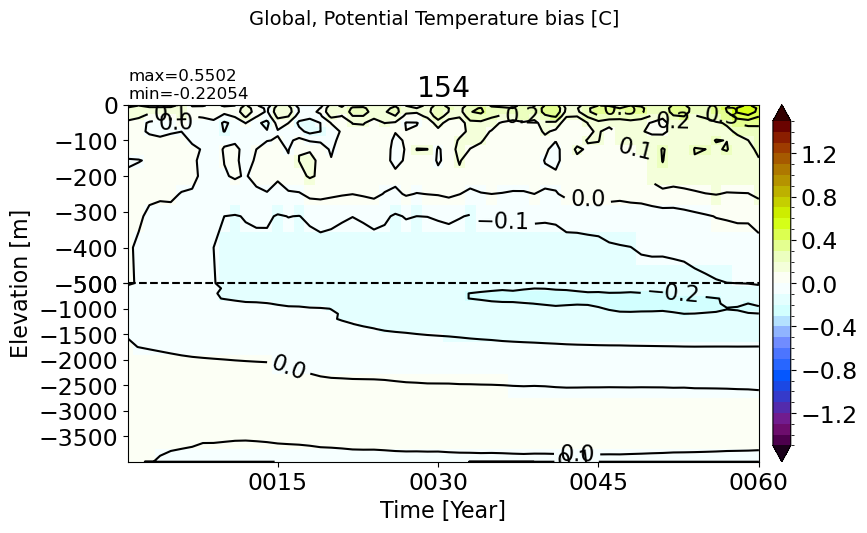
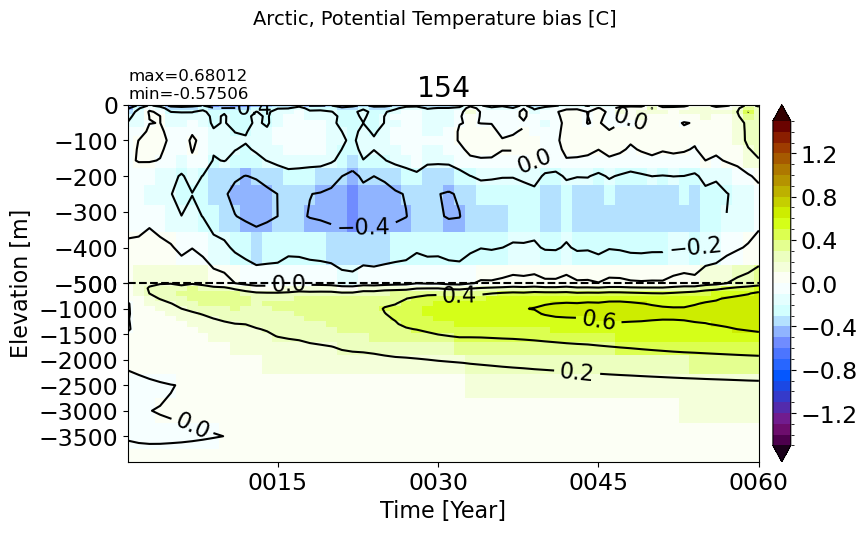
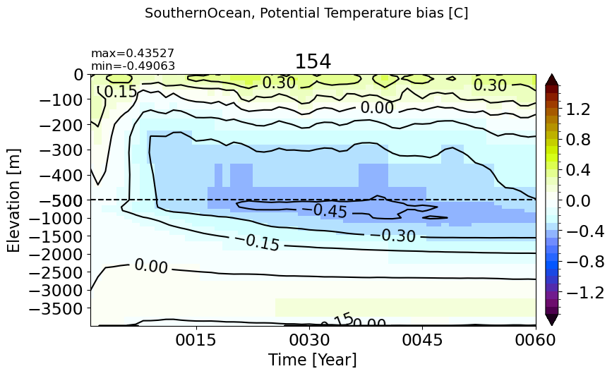
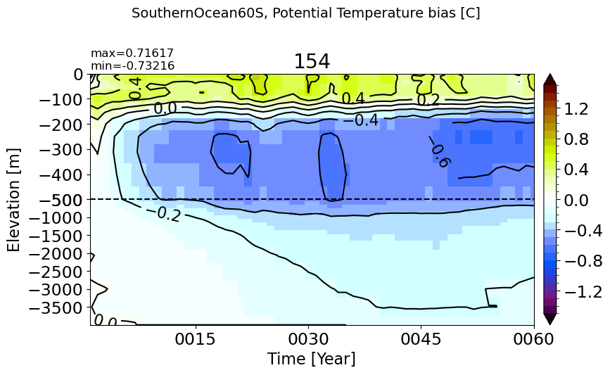
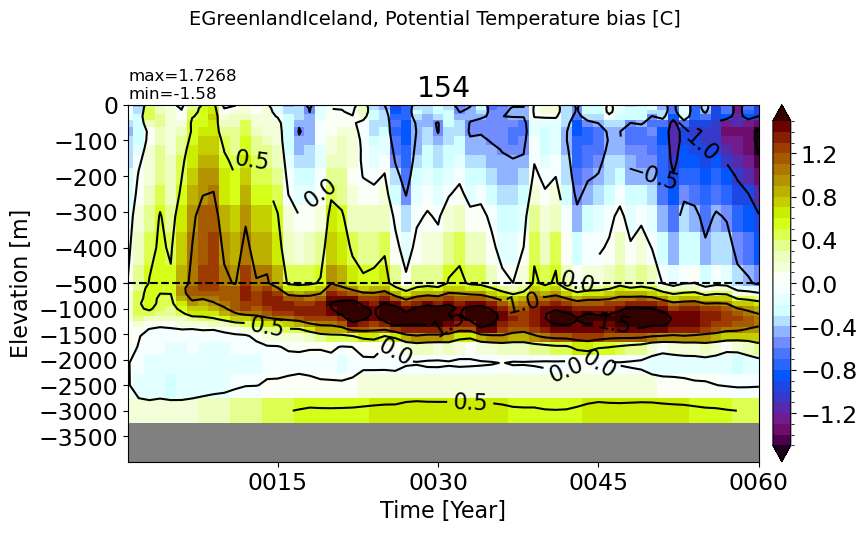
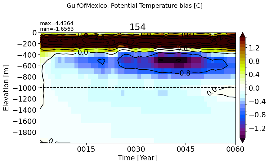
def make_temp_drift_plot(m='Global', vmax=1.5, splitscale =  [0., -500., -4000]):
  vmin=-vmax  
  for path, case, i in zip(ocn_path, casename, range(len(casename))):
    fig, ax = plt.subplots(nrows=nr, ncols=nc, figsize=fs, sharex=False, sharey=True)
    plt.suptitle(str(m)+', Potential Temperature bias [C]', fontsize=14)
    ds_mom = xr.open_dataset(path+case+'_thetao_drift.nc').sel(time=slice('0001-01-01', end_date))
    dummy_mom = np.ma.masked_invalid(ds_mom.sel(region=m).thetao_drift.values)
    ztplot(dummy_mom, ds_mom.time.values, ds_mom.z_l.values*-1, ignore=np.nan, splitscale=splitscale, 
           contour=True, axis=ax , title=label[i], extend='both', colormap='dunnePM', 
           autocenter=True, tunits='Year', show=False, clim=(vmin, vmax)) 
    plt.subplots_adjust(top = 0.8)
    plt.tight_layout()
      
  return

Global#

make_temp_drift_plot()

_images/ca67b4e8eb9fc92d0c12dead410c32d978021339cf1e7ddcb27f977ccd375611.png

Arctic#

make_temp_drift_plot(m='Arctic')

_images/e5369306de7df05304238b598fbe7677adbd195664dbcaa8fa36c75326056c19.png

SouthernOcean#

make_temp_drift_plot(m='SouthernOcean')

_images/aef11e95f07d820d3e52eb4987dce7671c20a731986b6170846da772e7048ff6.png

SouthernOcean60S#

make_temp_drift_plot(m='SouthernOcean60S')

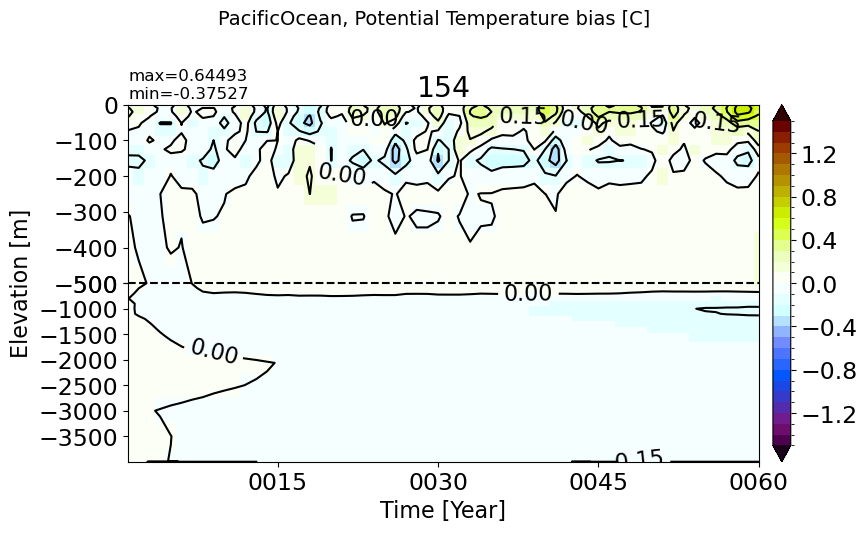
_images/5bb563e96ad4674b3b3dbc8f6a961cee27767f2d619b07ab509d528ba731b892.png

PacificOcean#

make_temp_drift_plot(m='PacificOcean')

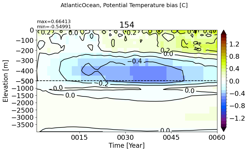
_images/5f422462fd7fc2896a0b74078314e06b6209e1a9749191984ea35e7c2a416e23.png

AtlanticOcean#

make_temp_drift_plot(m='AtlanticOcean')

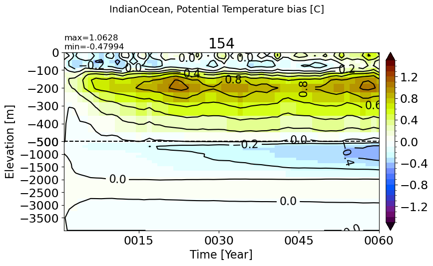
_images/986deecf8ed68ebcc72523b06fd7906a2983f3c10a2895de6e38783bf8531515.png

IndianOcean#

make_temp_drift_plot(m='IndianOcean')

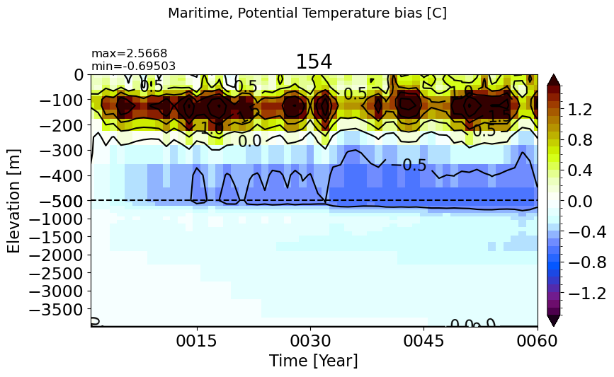
_images/283465d0f04fbefe8bce8cd72fbb9aaa9fcdbc06889bbefd32479b66dd6781a7.png

Maritime#

make_temp_drift_plot(m='Maritime')

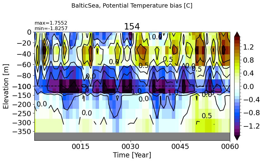
_images/da97981e3a34f7ca6ac0bc50baf2773caf8a4dc7547a9cfc3bd853b1b90250e3.png

BalticSea#

make_temp_drift_plot(m='BalticSea', splitscale =  [0., -100., -400])

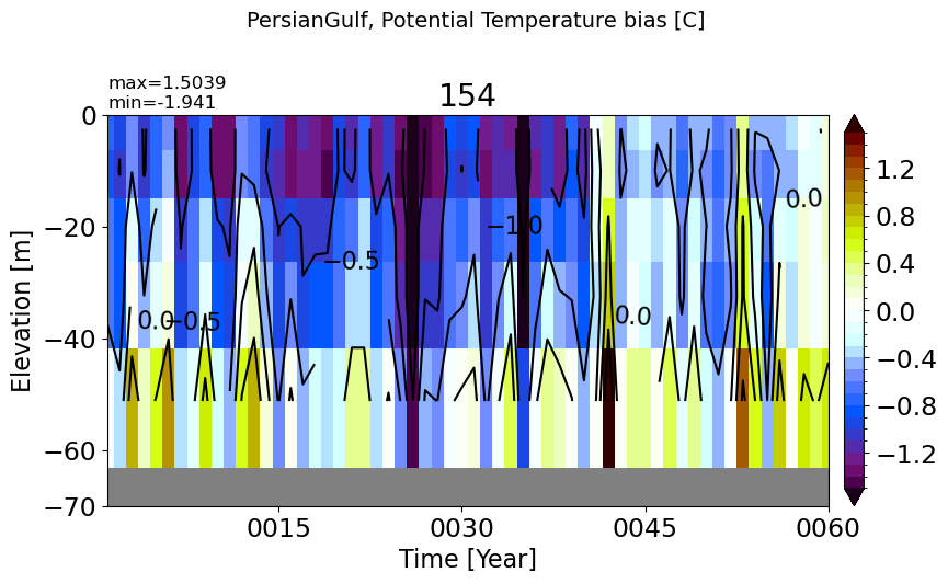
_images/c2bcdb78914df750ad73ed90f43b63f71c66bed1dca8add5ca9657765546013d.png

PersianGulf#

make_temp_drift_plot(m='PersianGulf', splitscale =  [0., -100., -70])

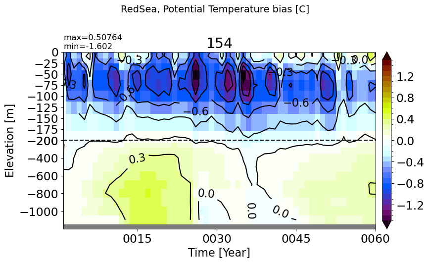
_images/274db2d624455ee2ed416bf040bda713b6d5489edefd68e0e961b7795faf8501.png

RedSea#

make_temp_drift_plot(m='RedSea', splitscale =  [0., -200., -1200])

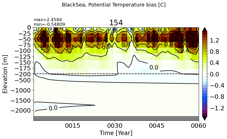
_images/bc22e0dbab944f26d5d021a5c941140644a345d1e589aea4bf1624d6d367dfea.png

BlackSea#

make_temp_drift_plot(m='BlackSea', splitscale =  [0., -200., -2500])

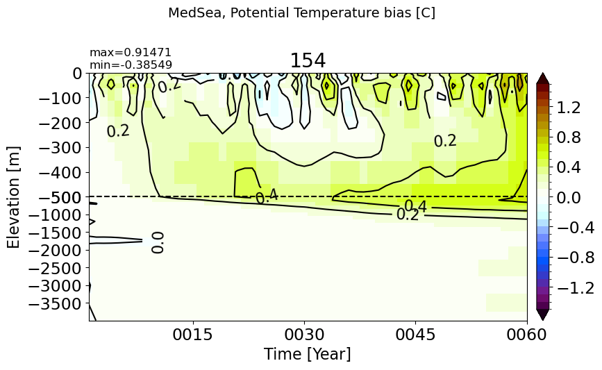
_images/2c8c21d0f41c00e33bc67c7f44b10fe9a2bd9c5affbab80fd672e1e6ed31754f.png

MedSea#

make_temp_drift_plot(m='MedSea')

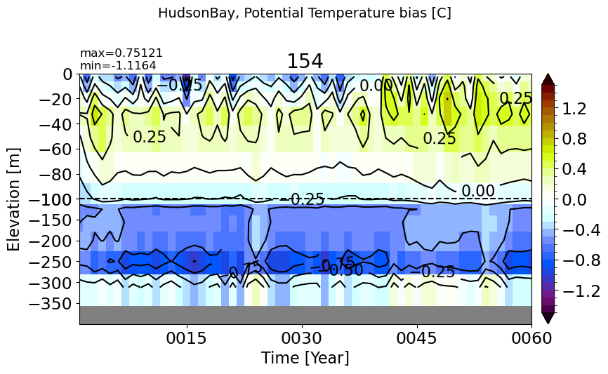
_images/94144c089153944da0d881bbf812ac7f769bb333d6eb14619fcd2dc1dd34adc9.png

HudsonBay#

make_temp_drift_plot(m='HudsonBay', splitscale =  [0., -100., -400])

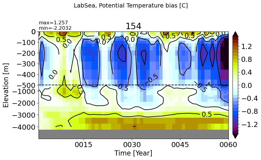
_images/a1a0f79cd0282e0ee4c750db9f2bddbca51fe196631b339cd52ec75f3c1568f6.png

LabSea#

make_temp_drift_plot(m='LabSea', splitscale =  [0., -500., -5000])

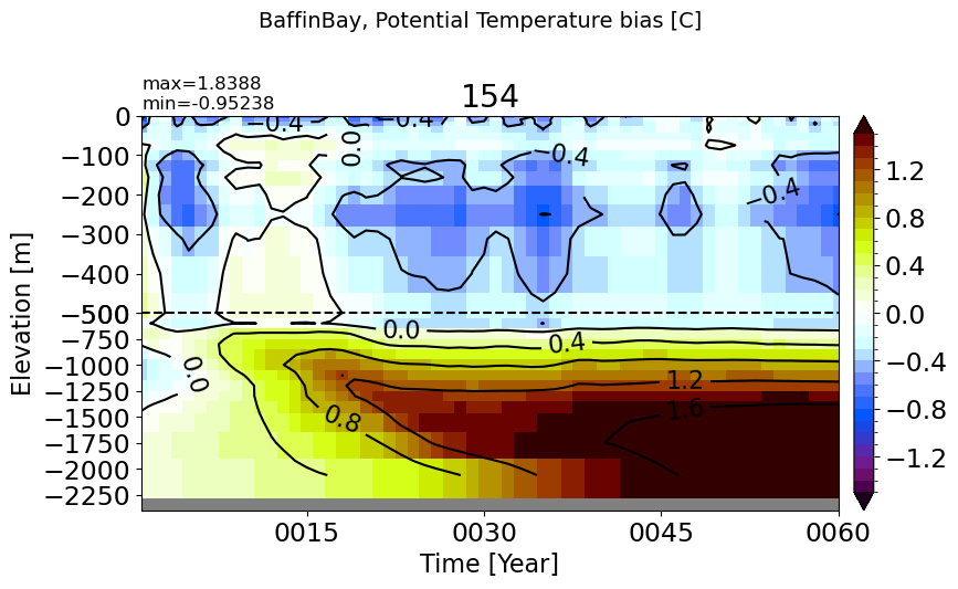
_images/f473eb09d89d7884048e22b4d27487d20c710a121e2cd18b3238c3cd3f102b75.png

BaffinBay#

make_temp_drift_plot(m='BaffinBay', splitscale =  [0., -500., -2400])

_images/3cbd83edce9defab2ad0f3528b2394dc139550f04294557e3a99df02421e3587.png

EGreenlandIceland#

make_temp_drift_plot(m='EGreenlandIceland')

_images/de61c97e45f359b08f208eb7a9a7533681afe5fec0158b53a31eee72ea11fdac.png

GulfOfMexico#

make_temp_drift_plot(m='GulfOfMexico', splitscale =  [0., -1000., -2000])

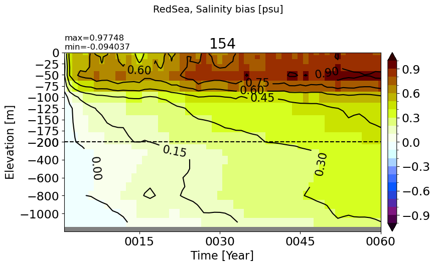
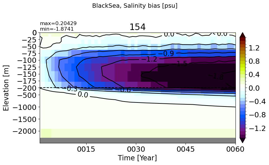
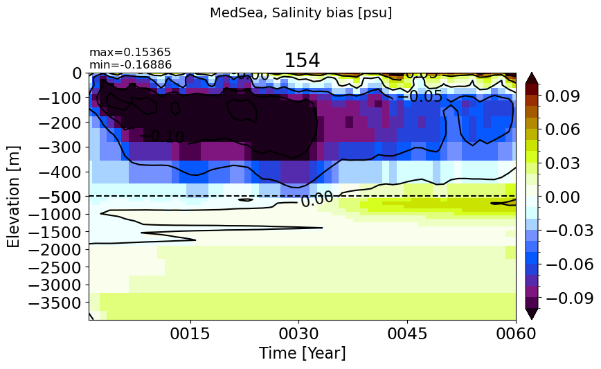
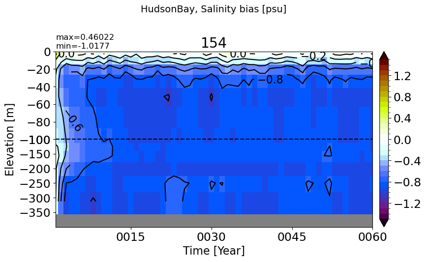
_images/a87db5a06a262984505e2d89f767ac5345f8b5fe245f982faceef07d6f578ad1.png

Salinity#

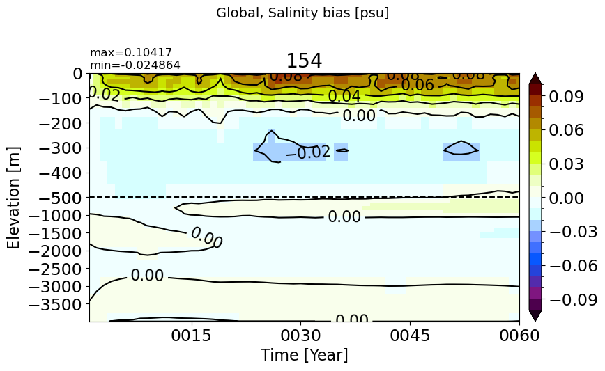
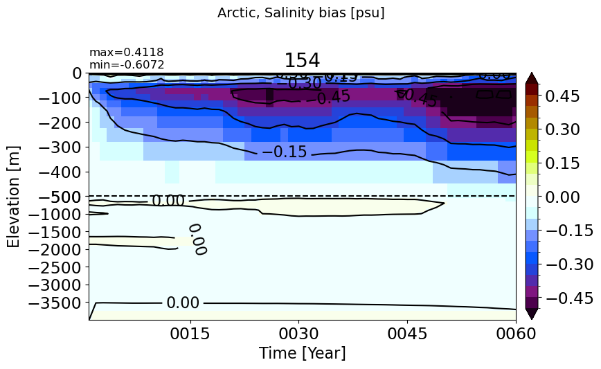
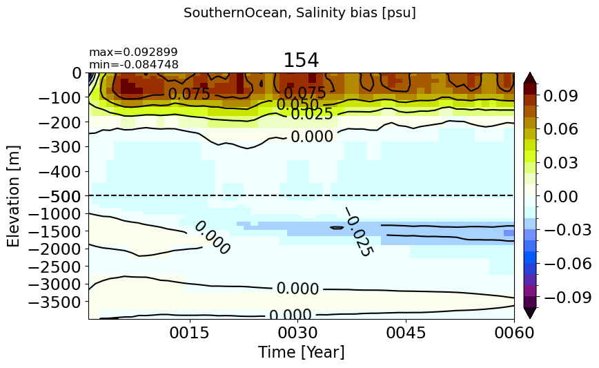
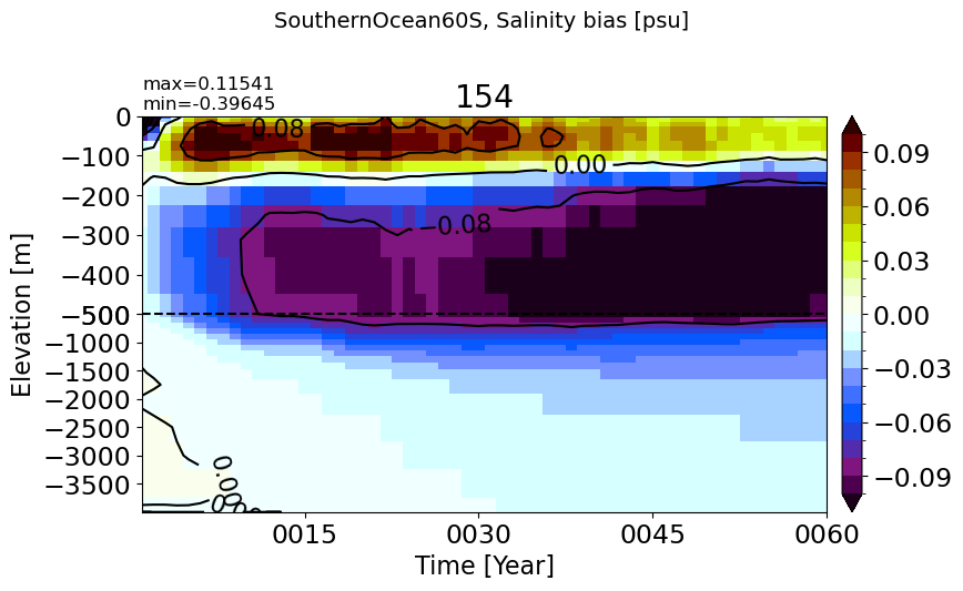
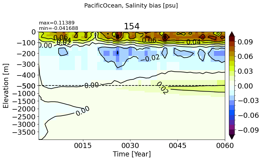
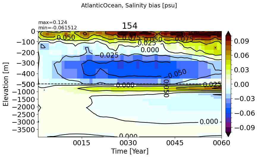
def make_salt_drift_plot(m='Global', vmax=0.1, splitscale=[0., -500., -4000]):
  vmin=-vmax
  for path, case, i in zip(ocn_path, casename, range(len(casename))):
    fig, ax = plt.subplots(nrows=nr, ncols=nc, figsize=fs, sharex=False, sharey=True)
    plt.suptitle(str(m)+', Salinity bias [psu]', fontsize=14)
    ds_mom = xr.open_dataset(path+case+'_so_drift.nc').sel(time=slice('0001-01-01', end_date))
    dummy_mom = np.ma.masked_invalid(ds_mom.sel(region=m).so_drift.values)
    ztplot(dummy_mom, ds_mom.time.values, ds_mom.z_l.values*-1, ignore=np.nan, splitscale=splitscale, 
           contour=True, axis=ax , title=label[i], extend='both', colormap='dunnePM', 
           autocenter=True, tunits='Year', show=False, clim=(vmin, vmax)) 
    plt.subplots_adjust(top = 0.8)
    plt.tight_layout()
  return

Global#

make_salt_drift_plot()

_images/7e7269eb283aa148f66d72d6776c26a6d1ea46b3ffb8db96e20bf88e1366ac04.png

Arctic#

make_salt_drift_plot(m='Arctic', vmax=0.5)

_images/73c76ac284c2958b6f93a13e557516290f315b03c90c2c3306635bf94bdf7cee.png

SouthernOcean#

make_salt_drift_plot(m='SouthernOcean')

_images/6d8ce263d4256515fd83bceb86f7e2c211680b8983a00b9755f64d1133432eae.png

SouthernOcean60S#

make_salt_drift_plot(m='SouthernOcean60S')

_images/8d312e0ed34b152819a026ac64e681c7c2c3735d8d9d04d5325249ea263769a7.png

PacificOcean#

make_salt_drift_plot(m='PacificOcean')

_images/0f34461e68b62c4cdd5cf80c387eb1ba8907a61318b110552915d65285c813ce.png

AtlanticOcean#

make_salt_drift_plot(m='AtlanticOcean')

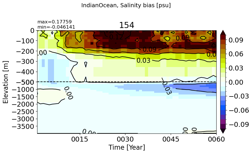
_images/bbe6d4fac9676d212ccd14fdd353a4acf978caff8397a789493a3fb618ef92c9.png

IndianOcean#

make_salt_drift_plot(m='IndianOcean')

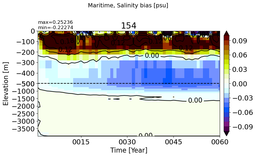
_images/8715c19260cbbcb35ea0e44edcd1af3b2f3a78355e6f7c7151d41ce229c0f36c.png

Maritime#

make_salt_drift_plot(m='Maritime')

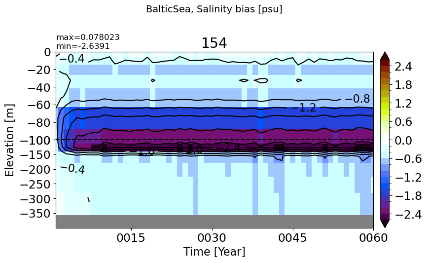
_images/24c8b8eab968e8e8508ae8139c2654e69fb5fa31f4ebf1c7e09a3fe33c8ed2db.png

BalticSea#

make_salt_drift_plot(m='BalticSea', vmax=2.5, splitscale =  [0., -100., -400])

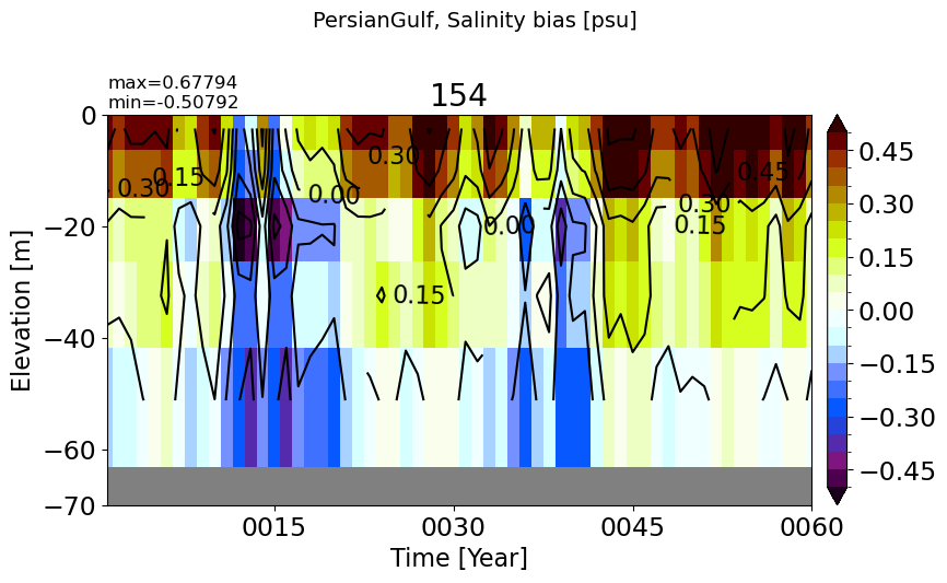
_images/fe3cc92097f6ea156f106c71382450a501e7c1d04fef9d0abcc710db07af85a9.png

PersianGulf#

make_salt_drift_plot(m='PersianGulf', vmax=0.5, splitscale =  [0., -100., -70])

_images/7859005c4fbf9c88d826793283895184de8489f3218e688e6842344e0ffde267.png

RedSea#

make_salt_drift_plot(m='RedSea', vmax=1.0, splitscale =  [0., -200., -1200])

_images/481346e9406d254f4e5582bef067eb57387ef4d7b7dcbbf43ff75b54464a9b02.png

BlackSea#

make_salt_drift_plot(m='BlackSea', vmax=1.5, splitscale =  [0., -200., -2500])

_images/2889d27bfcd5dfb605feb5d9a8f01db5cfb468de8ceb2f680e3871a68baf2c05.png

MedSea#

make_salt_drift_plot(m='MedSea')

_images/528270108b9f309ec75bad08ddd6bd6a6a7295cb0a546926a04bbb19e54caa54.png

HudsonBay#

make_salt_drift_plot(m='HudsonBay', vmax=1.5, splitscale =  [0., -100., -400])

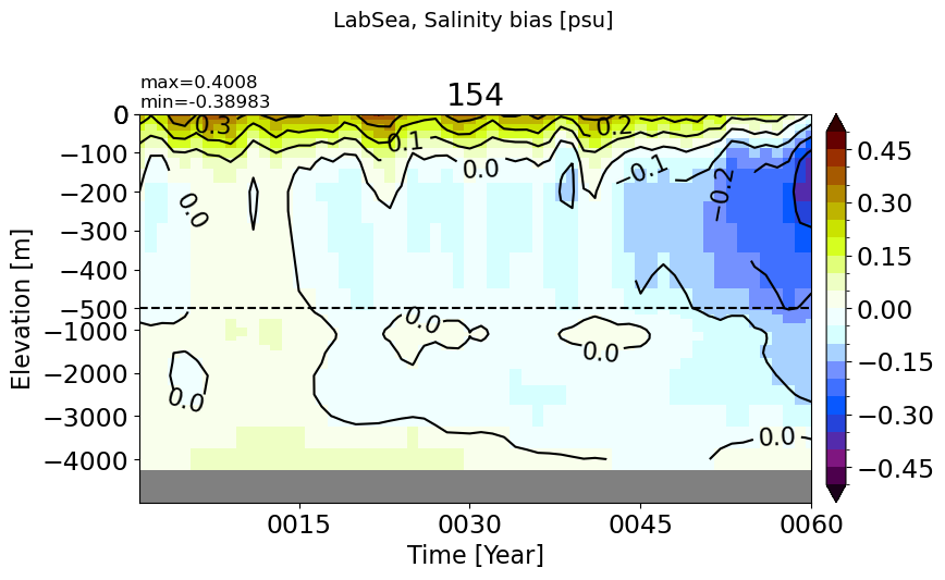
_images/9bbc88756f39d3cea78216fec2accc3976d94d71ad430a152724f5adc3165148.png

LabSea#

make_salt_drift_plot(m='LabSea', vmax=0.5, splitscale =  [0., -500., -5000])

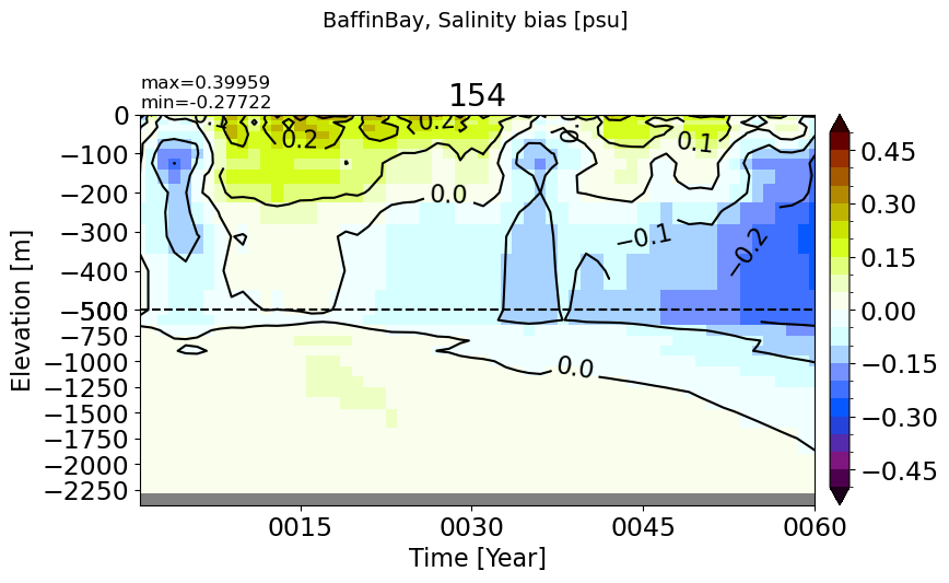
_images/9bb4755bb8072abb22e732083cd1361b14441598248231fb573c3b0f7a5b9980.png

BaffinBay#

make_salt_drift_plot(m='BaffinBay', vmax=0.5, splitscale =  [0., -500., -2400])

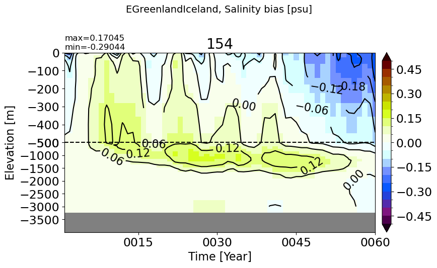
_images/6b37329f2ddb06ed408da8b061c6f131c58bb1b92705ffed05ed1cdaf3e6cd83.png

EGreenlandIceland#

make_salt_drift_plot(m='EGreenlandIceland', vmax=0.5)

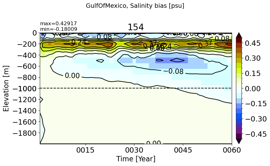
_images/0b40932b45676b14d9f689bdadb704f258ab299a0143ea6983d5b3bd91e5c6fe.png

GulfOfMexico#

make_salt_drift_plot(m='GulfOfMexico', vmax=0.5, splitscale =  [0., -1000., -2000])

_images/0467905be6bbcfa4827dfd435f14af1d828be99de75f9e231bba0f2da408cf51.png

RMSE#

Potential Temperature#

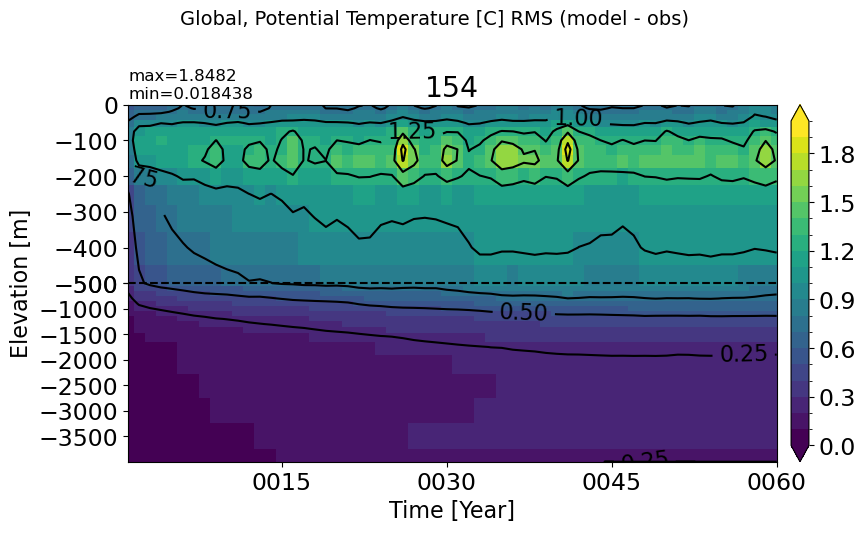
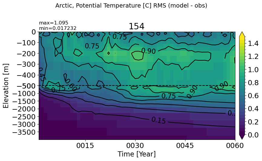
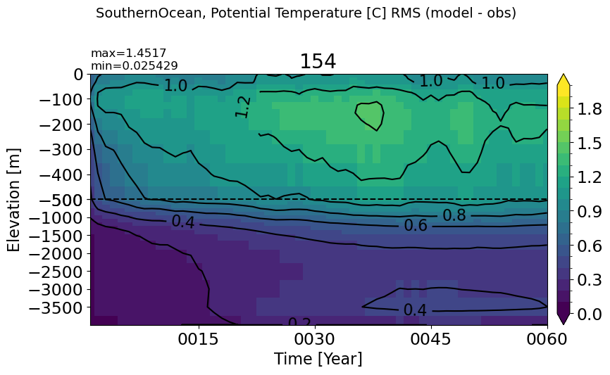
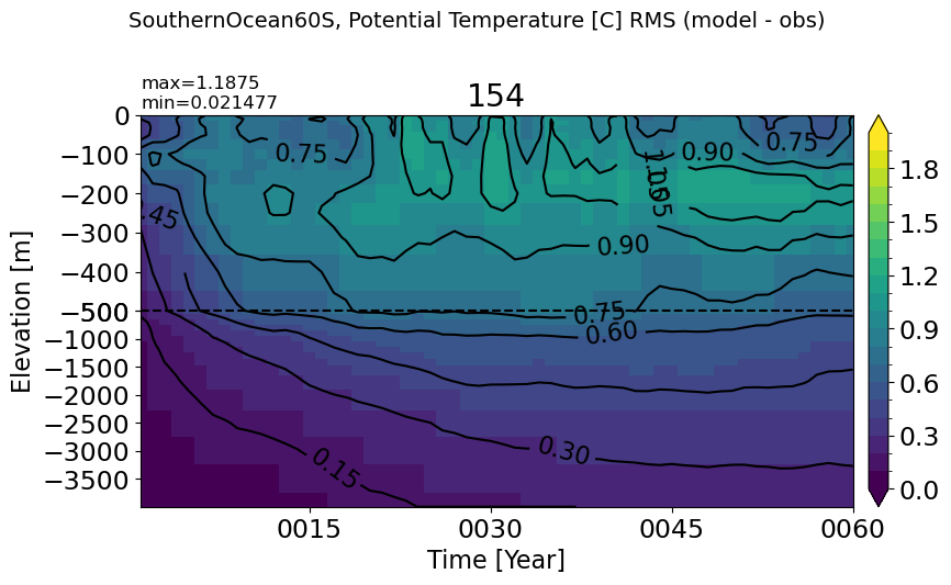
def make_temp_rmse_plot(m='Global', vmax=3, splitscale =  [0., -500., -4000]):
    vmin=0
    for path, case, i in zip(ocn_path, casename, range(len(casename))):
        fig, ax = plt.subplots(nrows=nr, ncols=nc, figsize=fs, sharex=False, sharey=True)
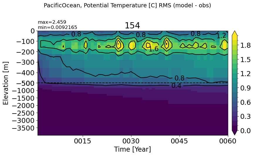
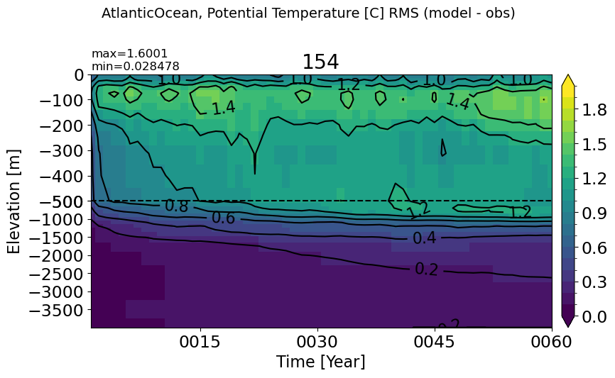
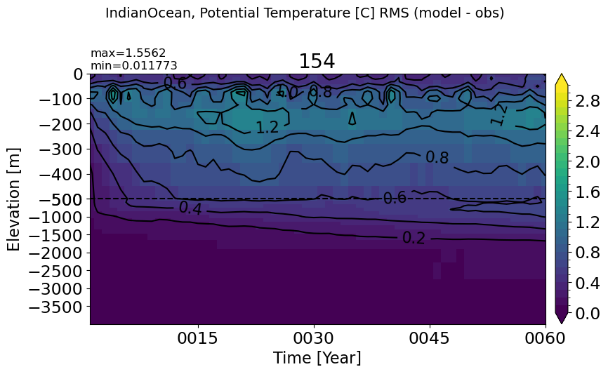
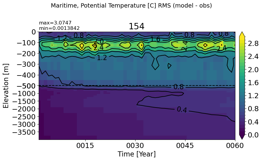
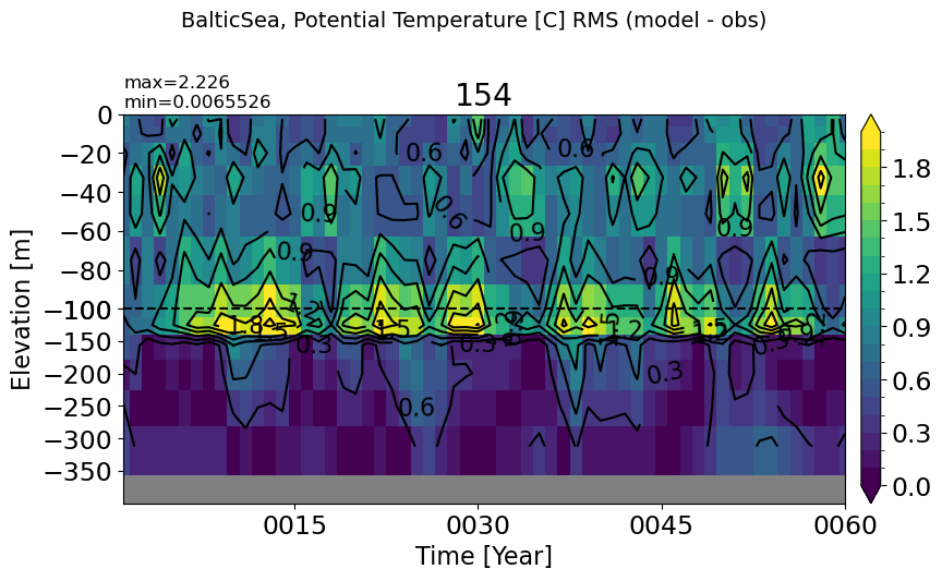
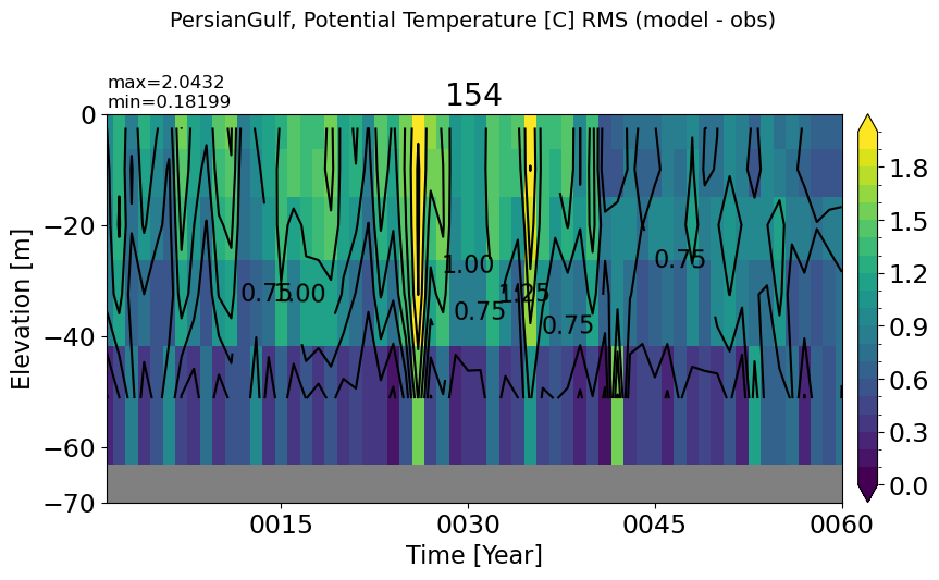
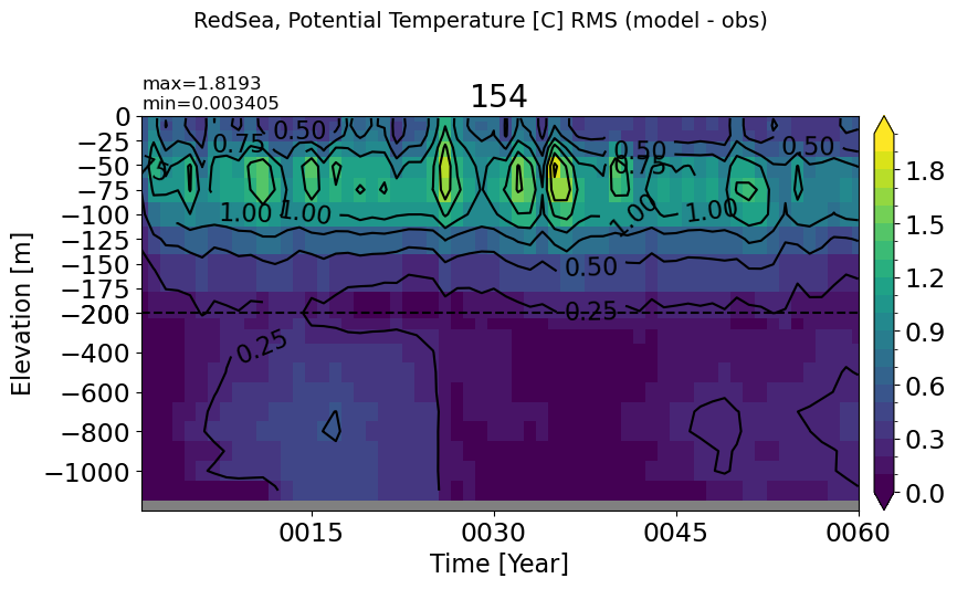
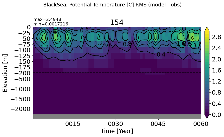
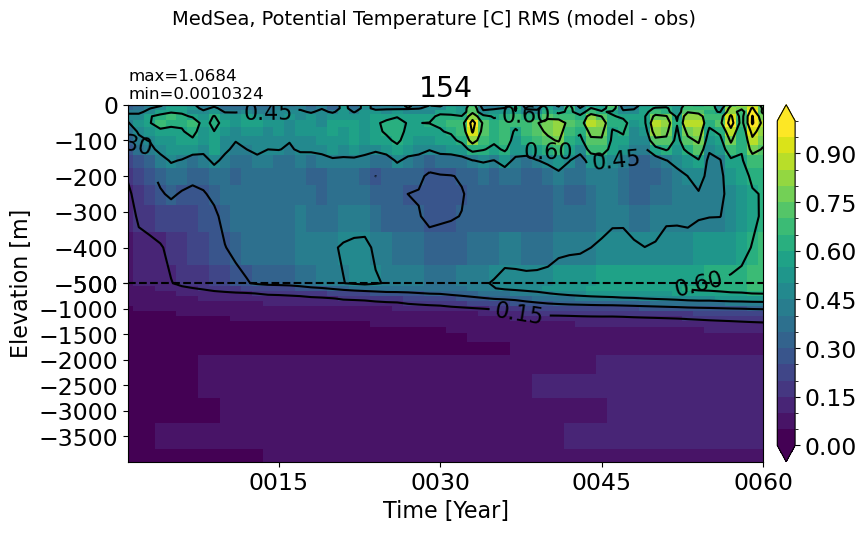
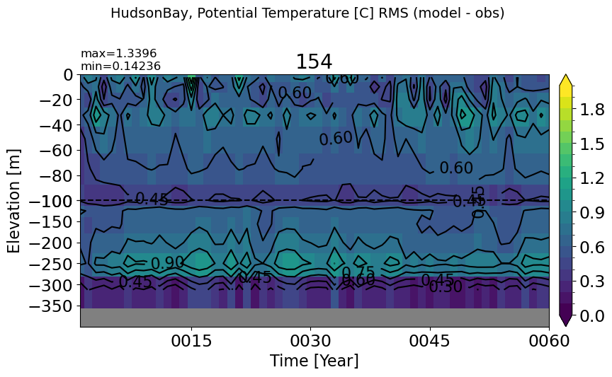
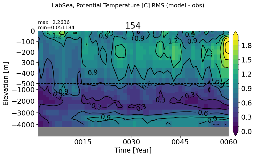
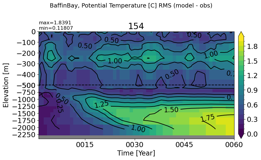
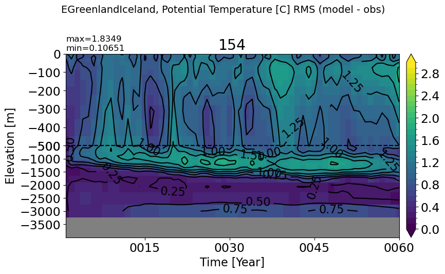
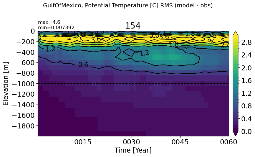
        plt.suptitle(str(m)+', Potential Temperature [C] RMS (model - obs)', fontsize=14)
        ds_mom = xr.open_dataset(path+case+'_thetao_rmse.nc').sel(time=slice('0001-01-01', end_date))
        dummy_mom = np.ma.masked_invalid(ds_mom.sel(region=m).thetao_rms.values)
        ztplot(dummy_mom, ds_mom.time.values, ds_mom.z_l.values*-1, ignore=np.nan, splitscale=splitscale, 
               contour=True, axis=ax , title=label[i], extend='both', colormap='viridis', 
               autocenter=True, tunits='Year', show=False, clim=(vmin, vmax)) 
        plt.subplots_adjust(top = 0.8)
        plt.tight_layout()
    return

Global#

make_temp_rmse_plot(vmax=2)

_images/851474ab849c01bd928ff7ac45030129f8c4a484358b151abba506cac7c03312.png

Arctic#

make_temp_rmse_plot(m='Arctic', vmax=1.5)

_images/91912cda679c4475ac6ca5b5d7df64792adf56db87a921ae5f4949b303746715.png

SouthernOcean#

make_temp_rmse_plot(m='SouthernOcean', vmax=2)

_images/9c28a792e1de84aede8cc669893b3008fbf8362359498517953f845f38e6a7ab.png

SouthernOcean60S#

make_temp_rmse_plot(m='SouthernOcean60S', vmax=2)

_images/fcecb7fc920d4a00bb98aadc8fbca054a16cf4cf25cac8e88a411ab7e19fd47b.png

PacificOcean#

make_temp_rmse_plot(m='PacificOcean', vmax=2)

_images/54a355bc3946265a02be49ffdb9cf4d1d4d3c96fecc3120688c6debed635d7bb.png

AtlanticOcean#

make_temp_rmse_plot(m='AtlanticOcean', vmax=2)

_images/eb422ef844c87db27850f697d9e6ff85d4709e6c5b839f54f1fdcdcbebdae8e1.png

IndianOcean#

make_temp_rmse_plot(m='IndianOcean')

_images/8aef8e46f526acfa5efb3424ce8f9b0ae22875e382483d43bc53fdbb411c6c62.png

Maritime#

make_temp_rmse_plot(m='Maritime')

_images/53512c3c8357271c5b167ee7179593283487b7ac5b72929fc7f967c440347db1.png

BalticSea#

make_temp_rmse_plot(m='BalticSea', vmax=2, splitscale =  [0., -100., -400])

_images/b3d0be9e676e9787f2973c998b39450c9f6fe32547584cf99fadf4beea06224f.png

PersianGulf#

make_temp_rmse_plot(m='PersianGulf', vmax=2,splitscale =  [0., -100., -70])

_images/a33bca8c5906e230d43bd0f716a16f415ab8659d66720fbdf4bcfce5b5c904f2.png

RedSea#

make_temp_rmse_plot(m='RedSea', vmax=2, splitscale =  [0., -200., -1200])

_images/099505cbea3d13810193c8e5a910559bd1afc1fa84c71aa00caec5c0707e5a3e.png

BlackSea#

make_temp_rmse_plot(m='BlackSea', splitscale =  [0., -200., -2500])

_images/8e9fe393df8dbb7367cdebea929095db68671466f9902a525ade57720aa81d80.png

MedSea#

make_temp_rmse_plot(m='MedSea', vmax=1)

_images/64de031d6ca61629ef9cea1f09f5ebf2ef81fde86e19ab507ea86d877dc002c6.png

HudsonBay#

make_temp_rmse_plot(m='HudsonBay', vmax=2, splitscale =  [0., -100., -400])

_images/4893a98055115ee1f2b86b7d46686f7c00d7036ff379e137a888cda9ffaab2e4.png

LabSea#

make_temp_rmse_plot(m='LabSea', vmax=2, splitscale =  [0., -500., -5000])

_images/d299f845358fb699f68d0f1fde2acfe97e1588eac332326a8291e3c457f816e0.png

BaffinBay#

make_temp_rmse_plot(m='BaffinBay', vmax=2, splitscale =  [0., -500., -2400])

_images/4abe78015780b3b11e6457c9685ea90795f9b8884bb852825276cdd1b5f5cc87.png

EGreenlandIceland#

make_temp_rmse_plot(m='EGreenlandIceland')

_images/0d3c59393236d9deef4fe2a74a4970ef3a781819c9c12a992ad61d56a261b9bb.png

GulfOfMexico#

make_temp_rmse_plot(m='GulfOfMexico', splitscale =  [0., -1000., -2000])

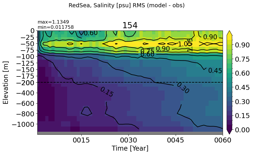
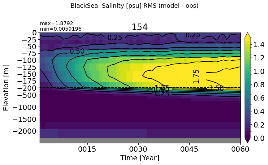
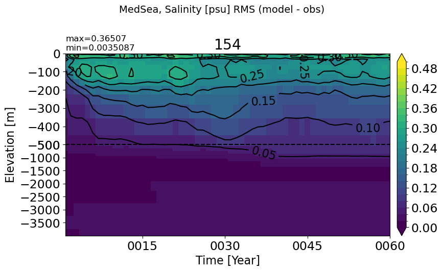
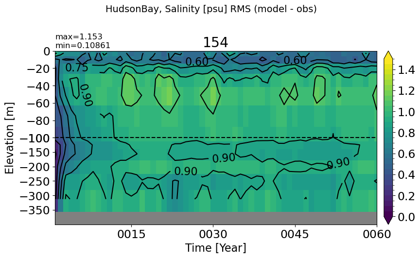
_images/b5adb8aa18176200758b17732deca65ffdddb36f62ee7891443f596fa1da7b2e.png

Salinity#

def make_salt_rmse_plot(m='Global', vmax=0.5, splitscale =  [0., -500., -4000]):
    vmin=0
    for path, case, i in zip(ocn_path, casename, range(len(casename))):
        fig, ax = plt.subplots(nrows=nr, ncols=nc, figsize=fs, sharex=False, sharey=True)
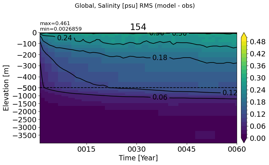
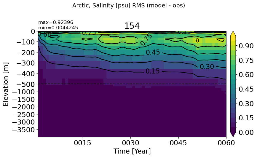
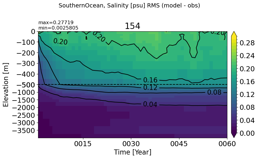
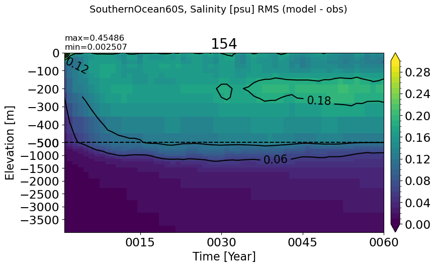
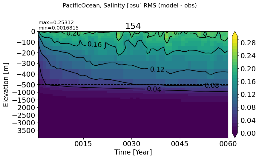
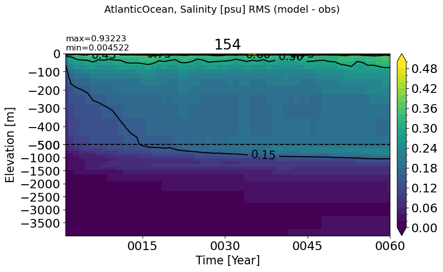
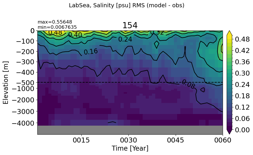
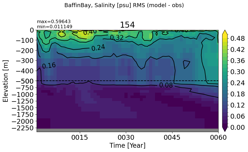
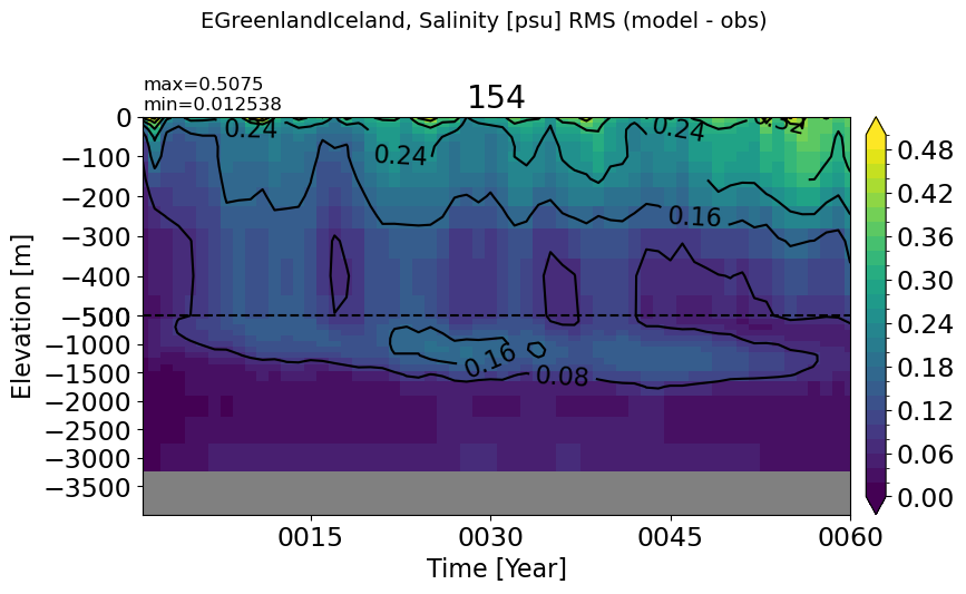
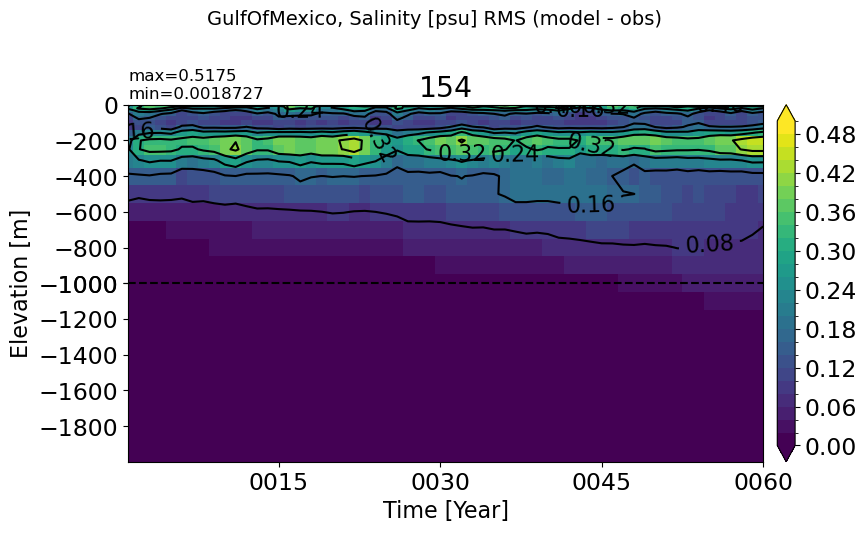
        plt.suptitle(str(m)+', Salinity [psu] RMS (model - obs)', fontsize=14)
        ds_mom = xr.open_dataset(path+case+'_so_rmse.nc').sel(time=slice('0001-01-01', end_date))
        dummy_mom = np.ma.masked_invalid(ds_mom.sel(region=m).so_rms.values)
        ztplot(dummy_mom, ds_mom.time.values, ds_mom.z_l.values*-1, ignore=np.nan, splitscale=splitscale, 
               contour=True, axis=ax , title=label[i], extend='both', colormap='viridis', 
               autocenter=True, tunits='Year', show=False, clim=(vmin, vmax)) 
        plt.subplots_adjust(top = 0.8)
        plt.tight_layout()
    return

Global#

make_salt_rmse_plot()

_images/2ac54514b280400cdd79f606b6146e4f224ced6dc7e1e62a0cda2ee0ad248ddd.png

Arctic#

make_salt_rmse_plot(m='Arctic', vmax=1)

_images/d00f0f7e9bff3f77e15352f602b074155a4ba92e9a54d2591d7ddf8099aa8187.png

SouthernOcean#

make_salt_rmse_plot(m='SouthernOcean', vmax=0.3)

_images/dd88850ac575fb07930621130cdb20ca781dc58edd1dbceab7c31947916d2a0c.png

SouthernOcean60S#

make_salt_rmse_plot(m='SouthernOcean60S', vmax=0.3)

_images/6a2c475d4aa8325b55d5728c146d590dd18c4b2df481769552994add38397521.png

PacificOcean#

make_salt_rmse_plot(m='PacificOcean', vmax=0.3)

_images/19d690d339de96021abe74328be644427936f6c9797fefa5cc1a4e48b2997470.png

AtlanticOcean#

make_salt_rmse_plot(m='AtlanticOcean')

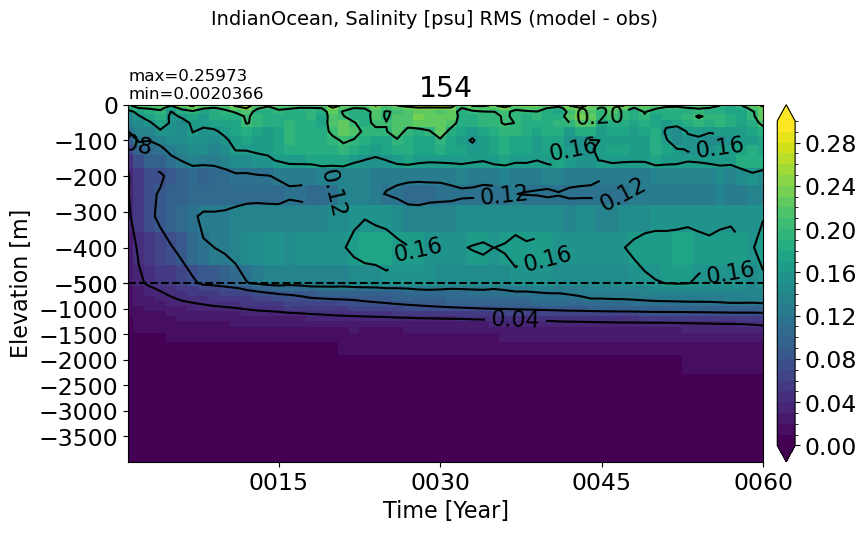
_images/745ba46f35c00259a8c797b08152e9234dac9521d7ddf9a0eb698f1b5ff982ca.png

IndianOcean#

make_salt_rmse_plot(m='IndianOcean', vmax=0.3)

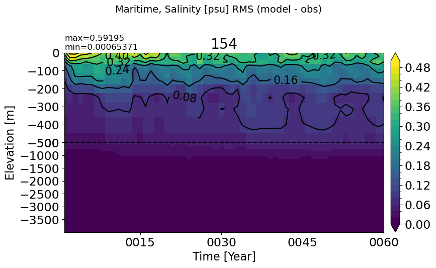
_images/17edf2a9263ae5b62110fedce2491f33ef7c65f80b1d97828cc20f4f1c4aec83.png

Maritime#

make_salt_rmse_plot(m='Maritime')

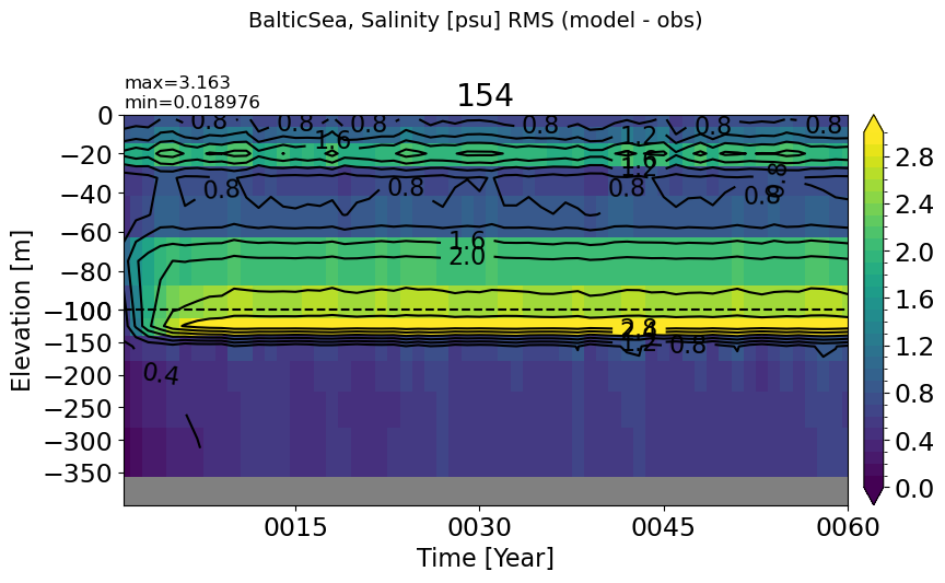
_images/2baed730b85fc7388c4f08ffdf85ef80efa1058f087b8b115b5d7c940a4541e2.png

BalticSea#

make_salt_rmse_plot(m='BalticSea', vmax=3, splitscale =  [0., -100., -400])

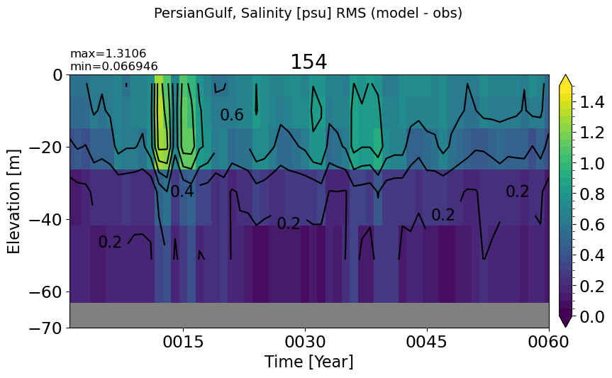
_images/544b5e63a709e5afe365bc5148d916f609548ce76716279db1b700732b2bcad5.png

PersianGulf#

make_salt_rmse_plot(m='PersianGulf', vmax=1.5, splitscale =  [0., -100., -70])

_images/c642e88bcfff6401c0e64272a012349e0013302f281e4a5471da8d7712865db6.png

RedSea#

make_salt_rmse_plot(m='RedSea', vmax=1.0, splitscale =  [0., -200., -1200])

_images/eaeb4b834a78e8aff30a24a7f801d1895c78c32c2bd679941508d783ae92b6c9.png

BlackSea#

make_salt_rmse_plot(m='BlackSea', vmax=1.5, splitscale =  [0., -200., -2500])

_images/8224a005b54ebf83826863e3343a735cb5555f00147a092a610a39cd86758a8b.png

MedSea#

make_salt_rmse_plot(m='MedSea')

_images/23a9050382d80c53d76166c79c46e5024fb938ada05968a776374fe66b0b65fc.png

HudsonBay#

make_salt_rmse_plot(m='HudsonBay', vmax=1.5, splitscale =  [0., -100., -400])

_images/da10be1ba0573c4abc74649f7c34fde412340e999c931571bc4d93027b0c0411.png

LabSea#

make_salt_rmse_plot(m='LabSea', vmax=0.5, splitscale =  [0., -500., -5000])

_images/3249d75a660f2633d13162c0a2d3195a66098590f0173ca1b02da7084b4d513b.png

BaffinBay#

make_salt_rmse_plot(m='BaffinBay', vmax=0.5, splitscale =  [0., -500., -2400])

_images/4d3aa9567f81ad05e41812f748a8b75aa842c313c0230ef852c97c87f87ae4aa.png

EGreenlandIceland#

make_salt_rmse_plot(m='EGreenlandIceland')

_images/700e74725b6d5a2655509b8423474bc41dd941415e698960ef1da3ad5084458c.png

GulfOfMexico#

make_salt_rmse_plot(m='GulfOfMexico', splitscale =  [0., -1000., -2000])

_images/9ce9085b2563f039d0f351900e7e3eb5ce18d221ede5f41b37c5688325ed1a6d.png

Biases at selected vertical levels#

Potential Temperature#

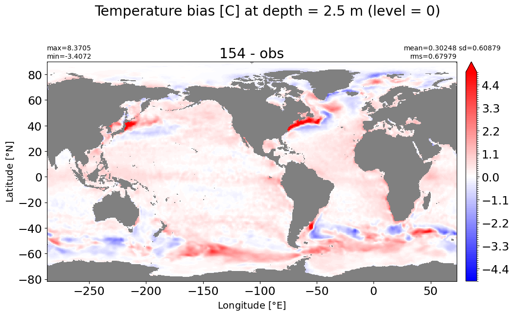
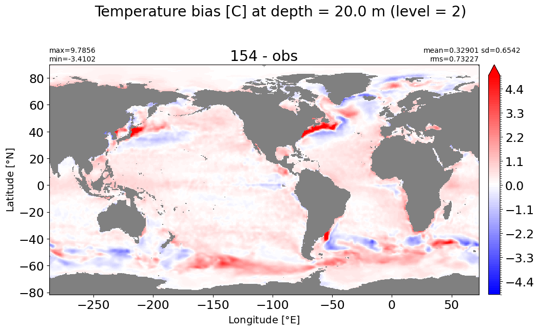
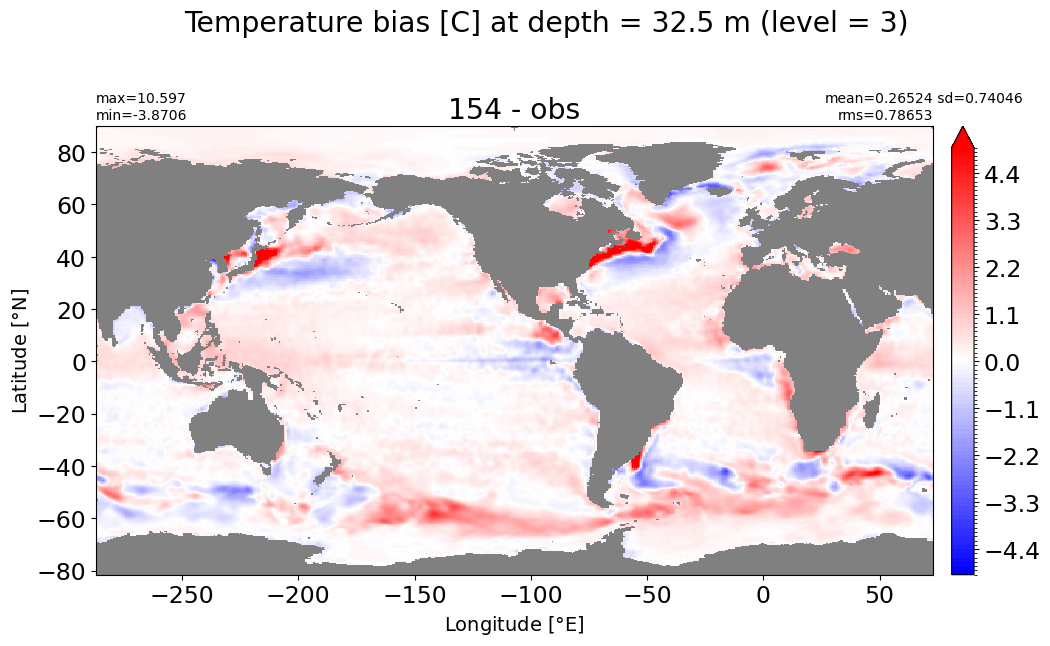
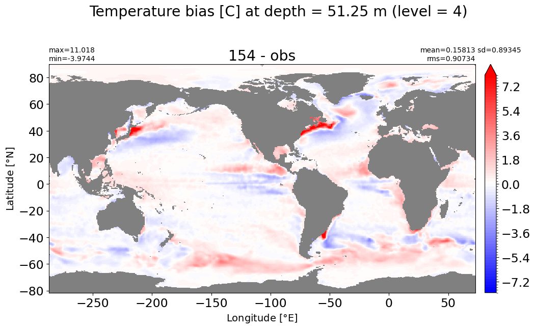
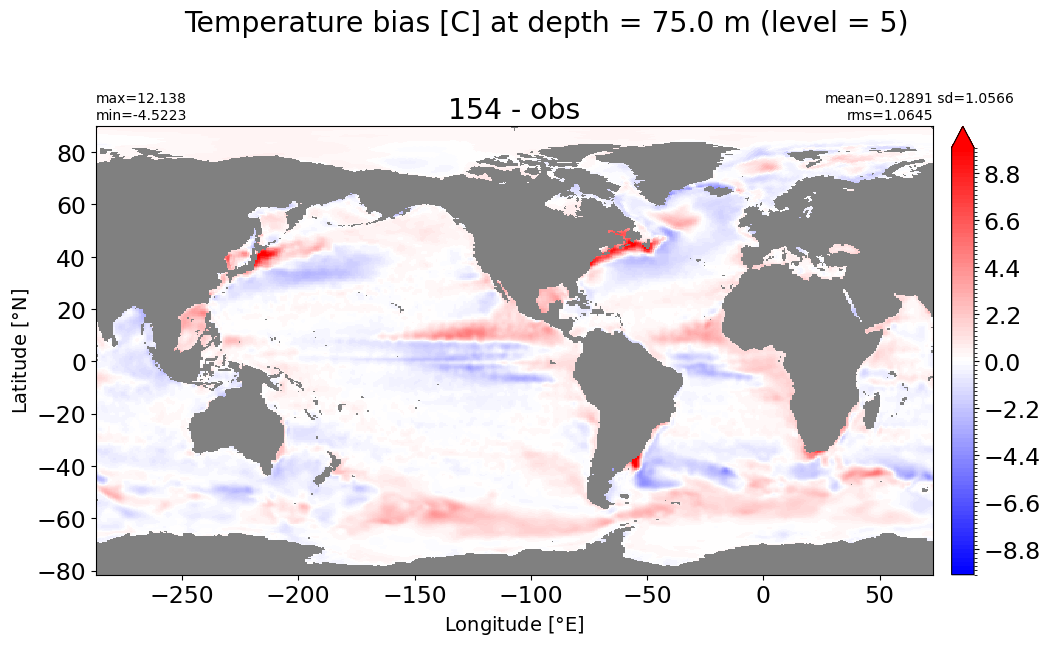
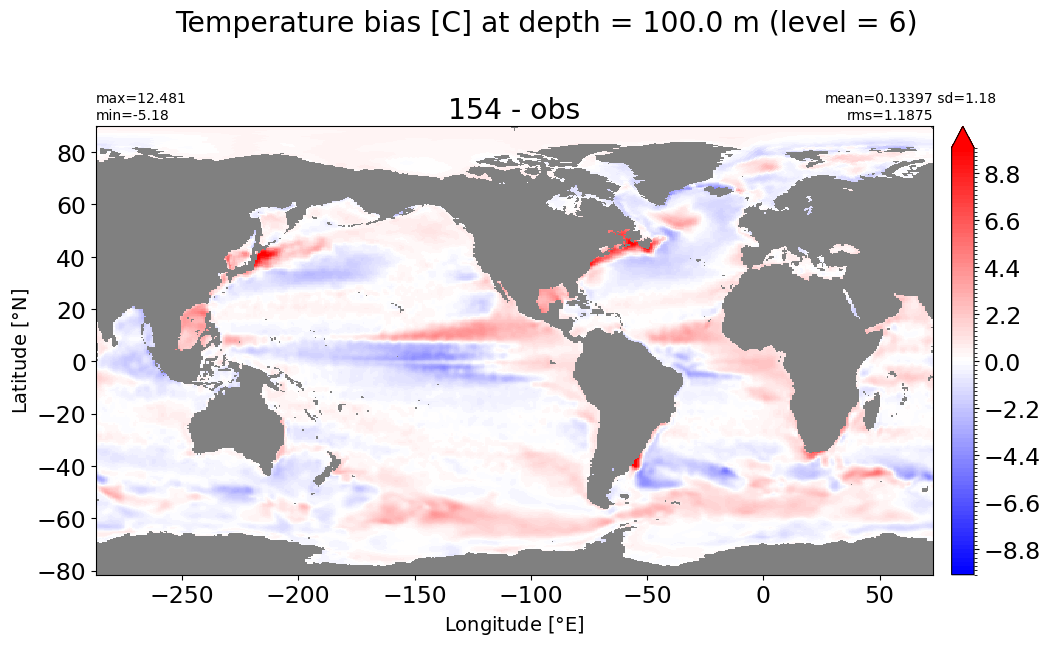
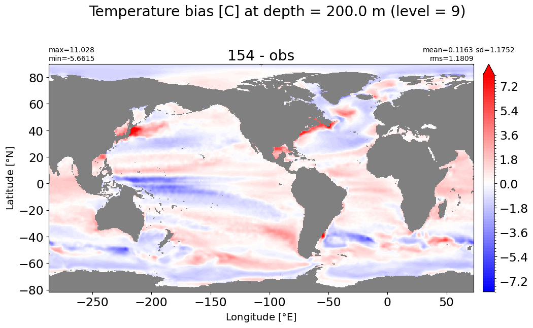
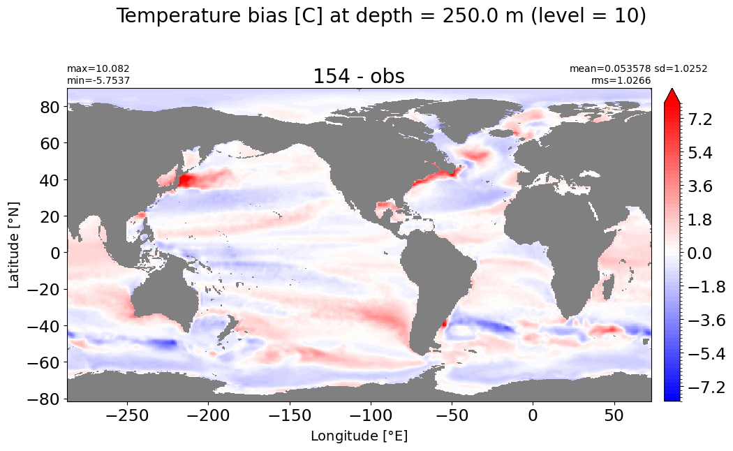
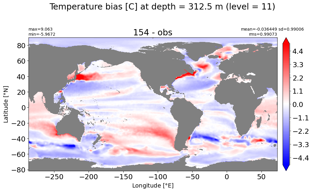
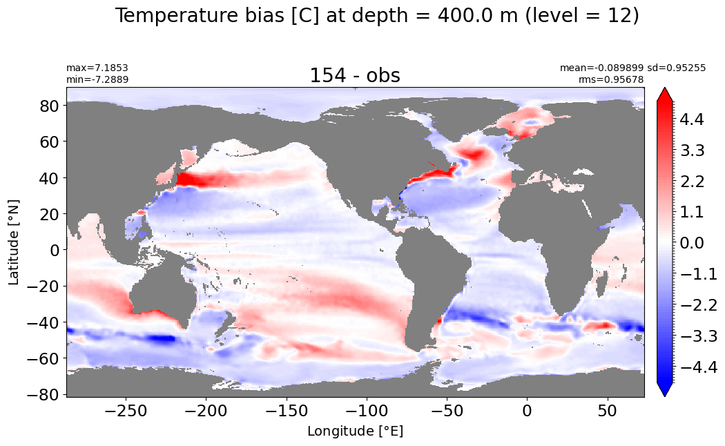
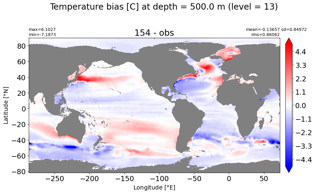
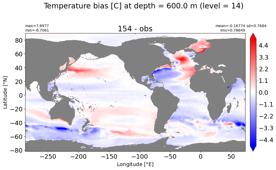
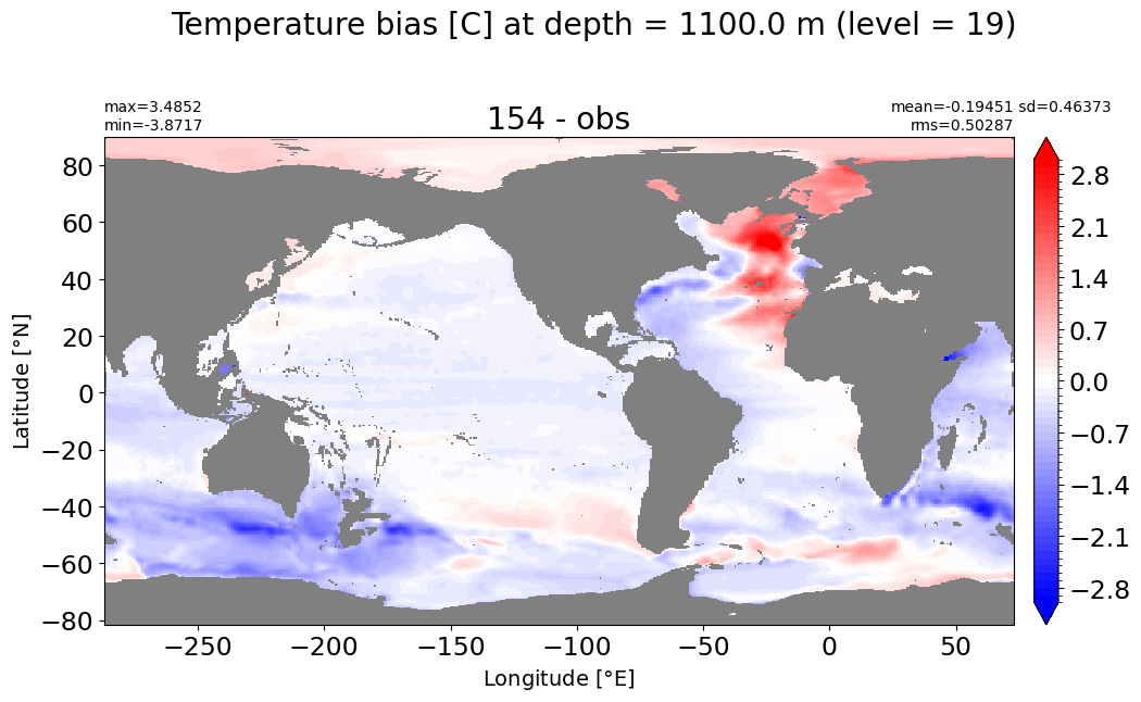
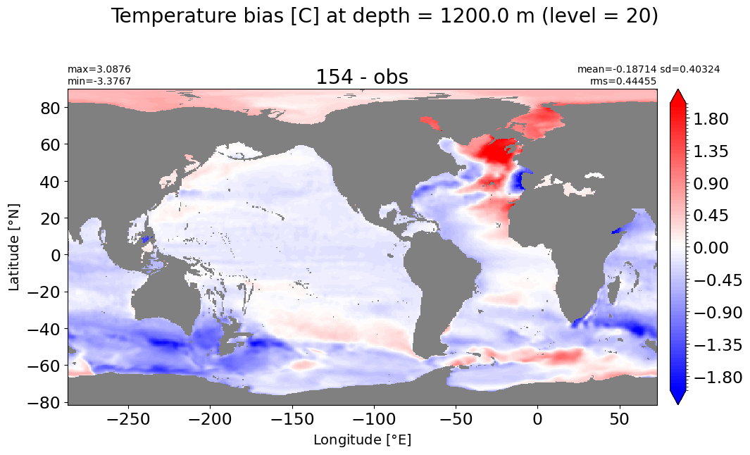
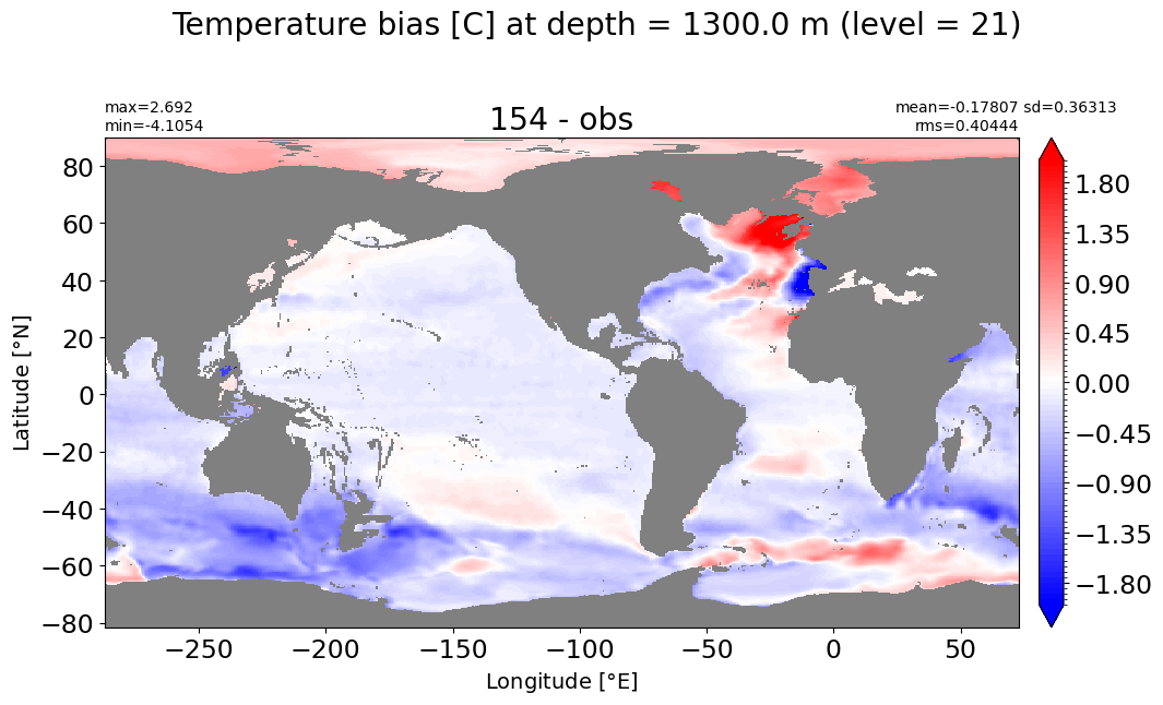
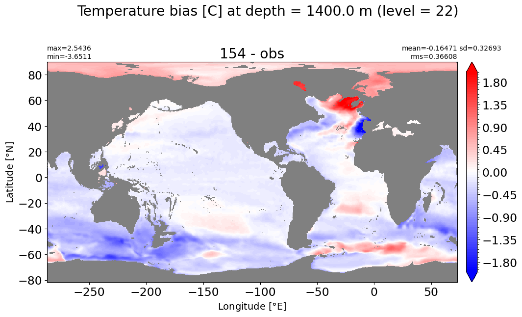
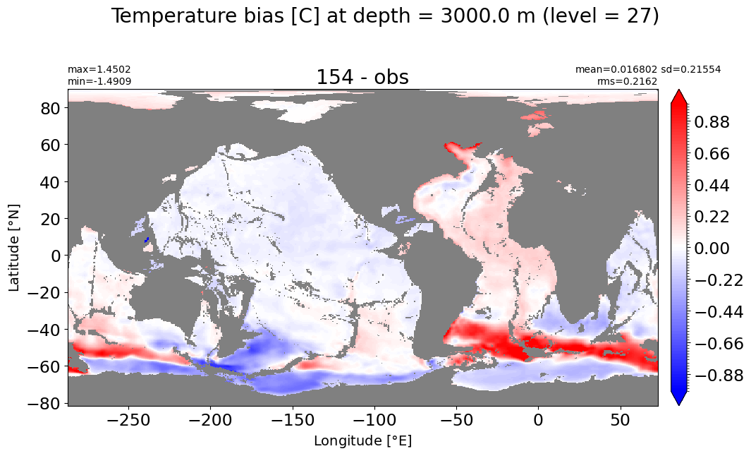
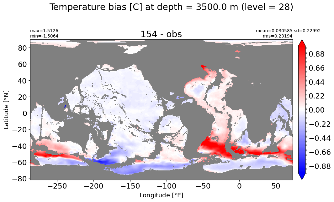
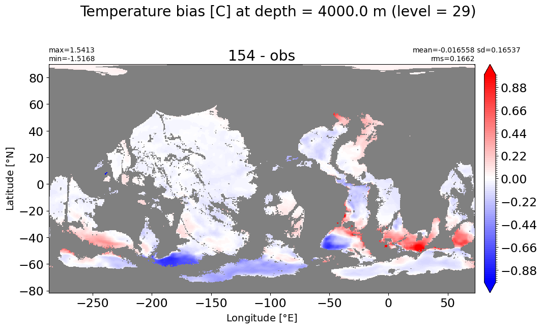
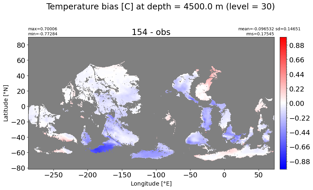
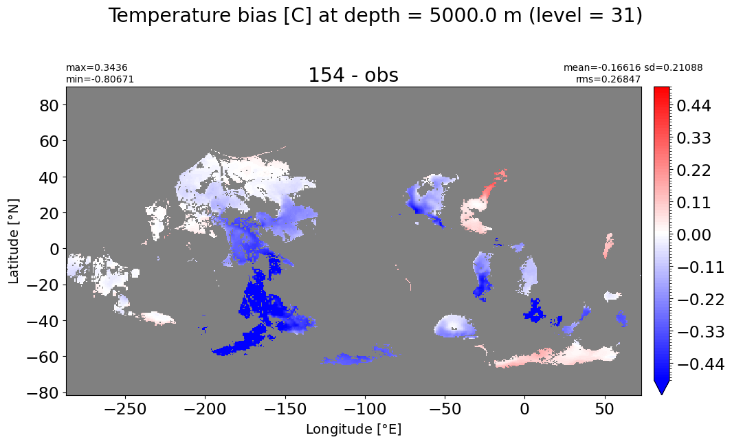
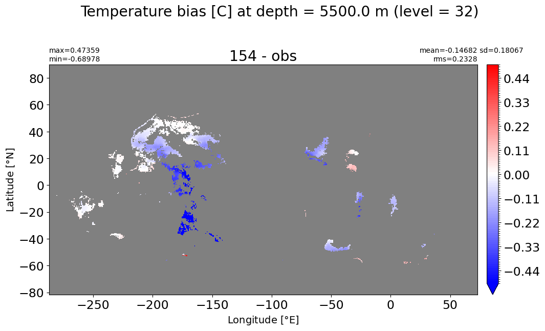
def make_temp_level_plot(k=0, t=5):
    for path, case, i in zip(ocn_path, casename, range(len(casename))):
        ds_mom_t = xr.open_dataset(path+case+'_thetao_time_mean.nc')
        if 'area_t' in dir(grd[i]):
          area = grd[i].area_t
        else:
          area = grd[i].areacello
        
        fig, ax = plt.subplots(nrows=1, ncols=1, figsize=(12,6.5))
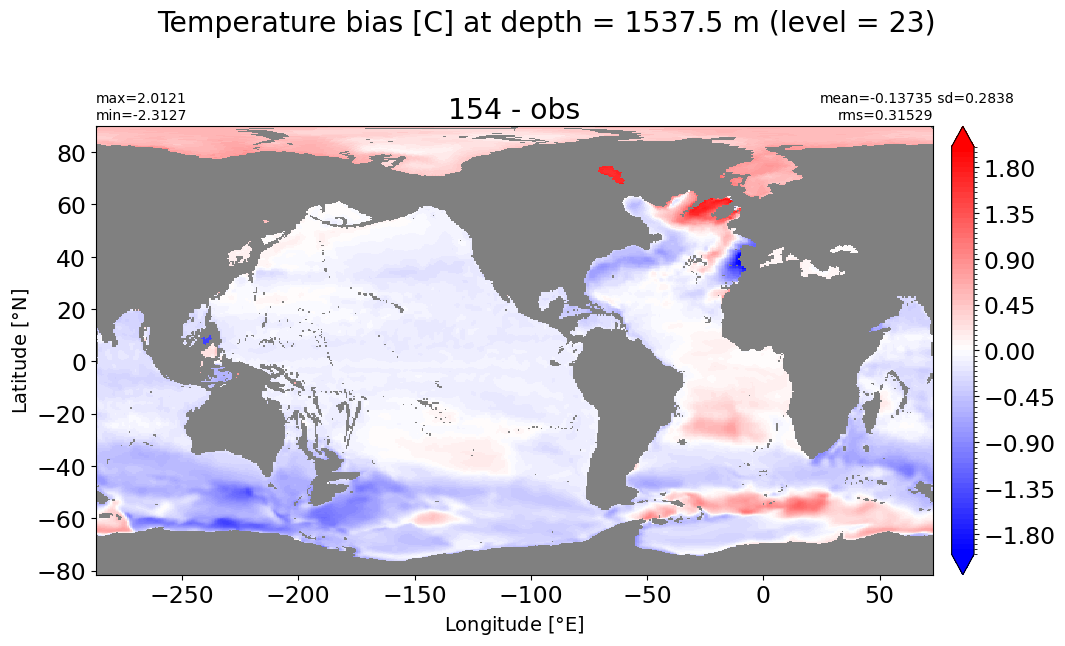
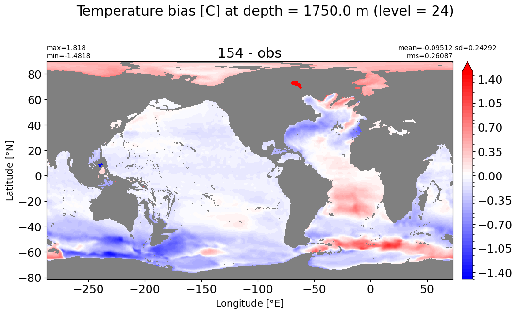
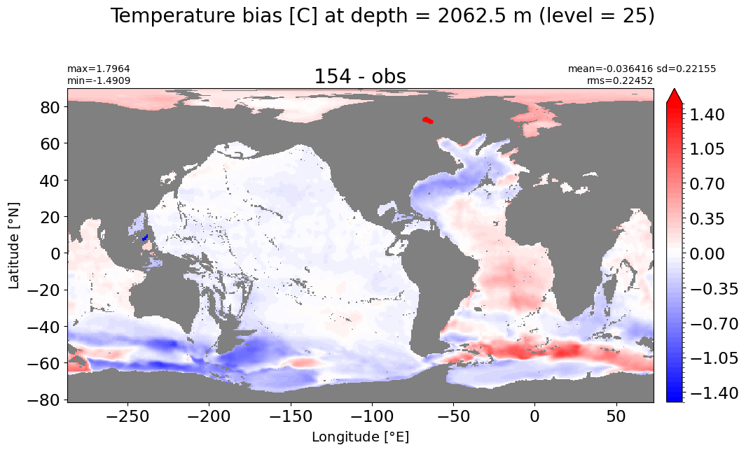
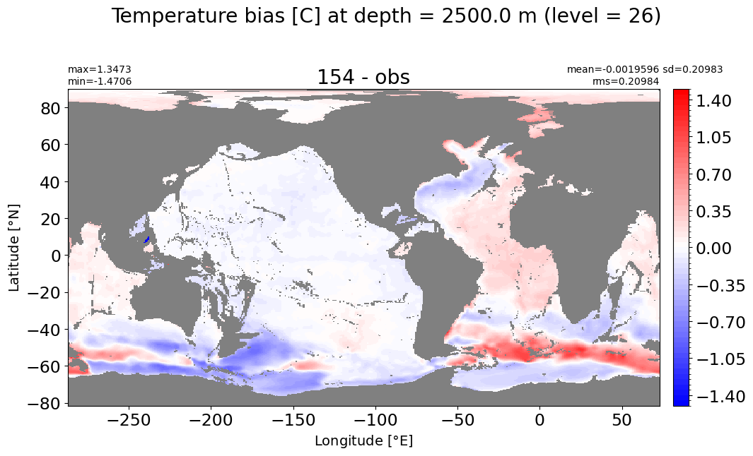
        temp_mom = np.ma.masked_invalid(ds_mom_t.thetao_bias[k,:].values)
        
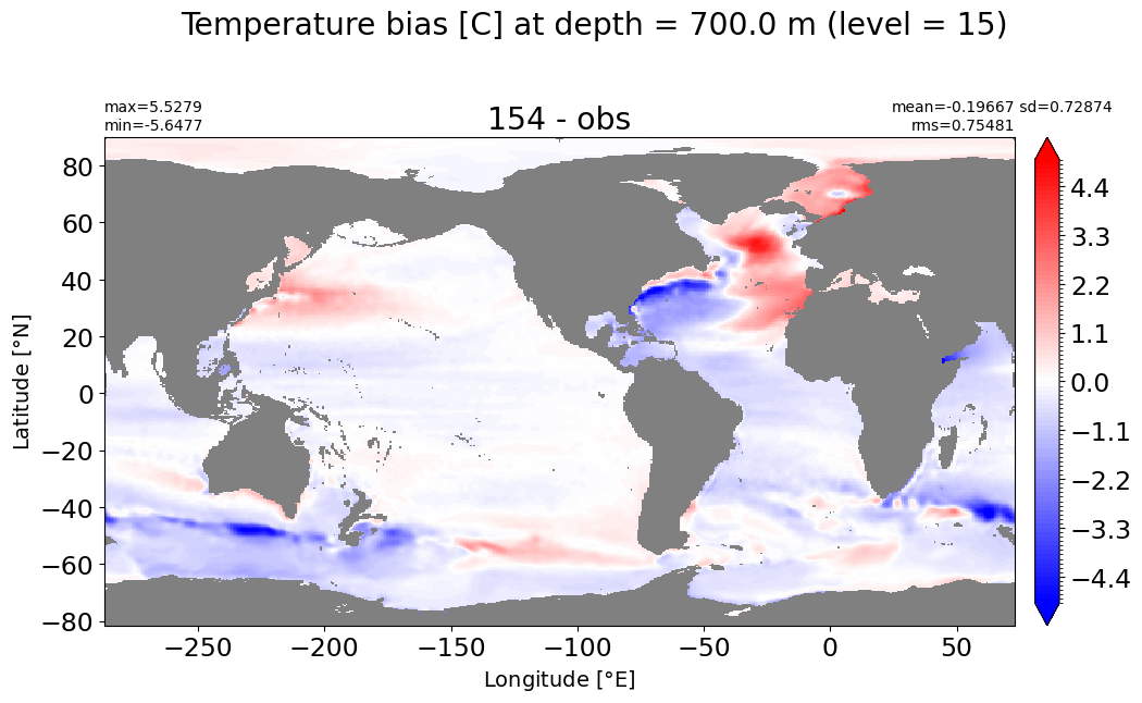
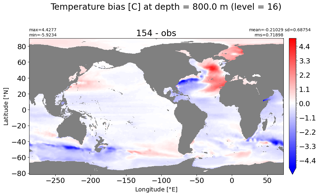
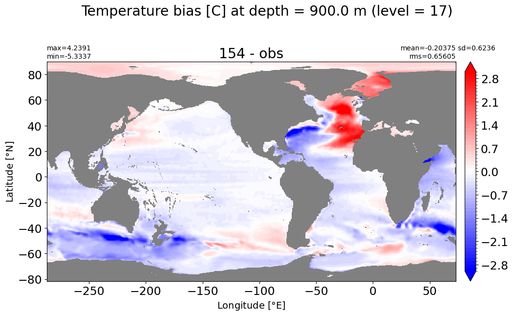
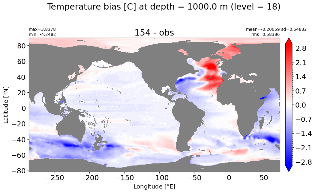
        plt.suptitle('Temperature bias [C] at depth = {} m (level = {})'.format(ds_mom_t.z_l[k].values, k))
        xyplot(temp_mom, grd[i].geolon, grd[i].geolat, area, title=str(label[i]+' - obs'), axis=ax, 
             clim=(-t,t), nbins=100, colormap=plt.cm.bwr, centerlabels=True)
        plt.subplots_adjust(top = 0.8)
    return

Depth = 2.5 m, k=0#

make_temp_level_plot(k=0, t=5)

_images/baf953f88fee74f859fa44d5edfeaa7039c31b916bfa18c75a1820fb884889f3.png

Depth = 10 m, k=1#

make_temp_level_plot(k=1, t=5)

_images/ada4223601d319084d142271e8f46f468b24247c1151b657d463e4b731f425f1.png

Depth = 20 m, k=2#

make_temp_level_plot(k=2, t=5)

_images/eda5587855eb34d6698a8ad57f5ca504c8f62f172885e1cf453a489c595620fc.png

Depth = 32.5 m, k=3#

make_temp_level_plot(k=3, t=5)

_images/9a4b6cbda6a3a5523ccab6ef1a26dd9f911dc3a677c487061f78f6d104d25dca.png

Depth = 51.25 m, k=4#

make_temp_level_plot(k=4, t=8)

_images/144ed2001526c2481b0d3d16b573555f073ca91ca6a3bc16a96c1a85d58caf74.png

Depth = 75 m, k=5#

make_temp_level_plot(k=5, t=10)

_images/997e9854338218c7be0e79f51741df9c508671cdc9d8afe7b9e4caa962aeb1af.png

Depth = 100 m, k=6#

make_temp_level_plot(k=6, t=10)

_images/5f4784521dd8768c2e34439effe2287fb06907e0b183506ad45789685b18f57b.png

Depth = 125 m, k=7#

make_temp_level_plot(k=7, t=10)

_images/64a66c461c35a2c33b2bd8d983ae3c3f3eee2586be90abc4e8709a0a890dd29f.png

Depth = 200 m, k=9#

make_temp_level_plot(k=9, t=8)

_images/a2968e4382f163fd1f7c3f9a64c6e914e232374b0d6b84c7bca86c695431b2f3.png

Depth = 250 m, k=10#

make_temp_level_plot(k=10, t=8)

_images/eb820b47c4a30f7624afe45c6f86a8d811b7f1e3a04db5ad0ef2eb3e6d84de82.png

Depth = 312.25 m, k=11#

make_temp_level_plot(k=11, t=5)

_images/5c7870d12a7bec33bcb54a97f321687473620f0963973a6c26b0276d4d790496.png

Depth = 400 m, k=12#

make_temp_level_plot(k=12, t=5)

_images/d8647457d6da5154bcaa677fcd3ba9af32f42d2b2afafe7393e46d3b7260db69.png

Depth = 500 m, k=13#

make_temp_level_plot(k=13, t=5)

_images/633b95391af28f51fa153165e0e610b9cb94d5c3ebf9210dc9672924eceda992.png

Depth = 600 m, k=14#

make_temp_level_plot(k=14, t=5)

_images/ab95ca81b20fceab8b93293af177a27e1f95d96f984dfb58e8d859a980f0e5b0.png

Depth = 700 m, k=15#

make_temp_level_plot(k=15, t=5)

_images/2da8042413c24b89ac3a77493cbfac548e75b9b287b8dc09c6ccb76665c6ebb3.png

Depth = 800 m, k=16#

make_temp_level_plot(k=16, t=5)

_images/bcb093b6ea2784aae54a4bca65a339f7663369c2813a113745a1d8a301171e27.png

Depth = 900 m, k=17#

make_temp_level_plot(k=17, t=3)

_images/e89e5c340b32f8ac8bb22a37fc440c15d9fa42ca79018f0d650f841cb4d59e21.png

Depth = 1000 m, k=18#

make_temp_level_plot(k=18, t=3)

_images/0fe966a9e256626f41d4220d2da442da49485aec996b62b7095fea8cd629dcfa.png

Depth = 1100 m, k=19#

make_temp_level_plot(k=19, t=3)

_images/68d47fb37fdfddfe59ecd283ef1a3ee31ddd93344d5b1e0bd05ab9342c19e838.png

Depth = 1200 m, k=20#

make_temp_level_plot(k=20, t=2)

_images/74dfe8ed5b732f17117f8da5d5dc18b0d0316e2e6976273cf98680619f8caf87.png

Depth = 1300 m, k=21#

make_temp_level_plot(k=21, t=2)

_images/df034ab59af3154fdbe8e9d4a9d751bef74277f126c83d0856fdaf9ef76277e8.png

Depth = 1400 m, k=22#

make_temp_level_plot(k=22, t=2)

_images/278db7c7a6eb35309599a945e7e03a9d15914ee07b799ac76f177f7da52aadcf.png

Depth = 1537.5 m, k=23#

make_temp_level_plot(k=23, t=2)

_images/c4ef66aa7270f1cd7cea96be474758ed26ec7054b680ccc0f13081e73881263f.png

Depth = 1750 m, k=24#

make_temp_level_plot(k=24, t=1.5)

_images/4b42f8eb7392c0a10619aa89c17964da19b69cca60fb9efc25c25db1b3d1c04d.png

Depth = 2062.5 m, k=25#

make_temp_level_plot(k=25, t=1.5)

_images/9bf4747d2282ed6db6fb1917935ee11faae3edd7a4c962f5c60ddd7a29bbc278.png

Depth = 2500 m, k=26#

make_temp_level_plot(k=26, t=1.5)

_images/aa06d9fd124b497b46528a9a010d4f4618d2a0c2617d29e1d259001ff72bce9c.png

Depth = 3000 m, k=27#

make_temp_level_plot(k=27, t=1.)

_images/7e228d6c2ba6d785d72cc756ae58d3b91109389fdf57dc18115417a480da8350.png

Depth = 3500 m, k=28#

make_temp_level_plot(k=28, t=1.)

_images/bebdc09b1f62ff9cb1799f6780cd729136d5e774ccc59128bca6671bcdfbdce6.png

Depth = 4000 m, k=29#

make_temp_level_plot(k=29, t=1)

_images/21c9c0316af172dcf6a700eca5773f07960d1d7859ded4aa7b7effea27aa9468.png

Depth = 4500 m, k=30#

make_temp_level_plot(k=30, t=1)

_images/7ec39d9046ed4e5ae83fb43196e12b83098d0b365c07c11d376a77a8881e950c.png

Depth = 5000 m, k=31#

make_temp_level_plot(k=31, t=0.5)

_images/9b3b32a4450e5c03bd1afc9c78d0bc05d3c9c134cb77d3dd1fa30320045b42fd.png

Depth = 5500 m, k=32#

make_temp_level_plot(k=32, t=0.5)

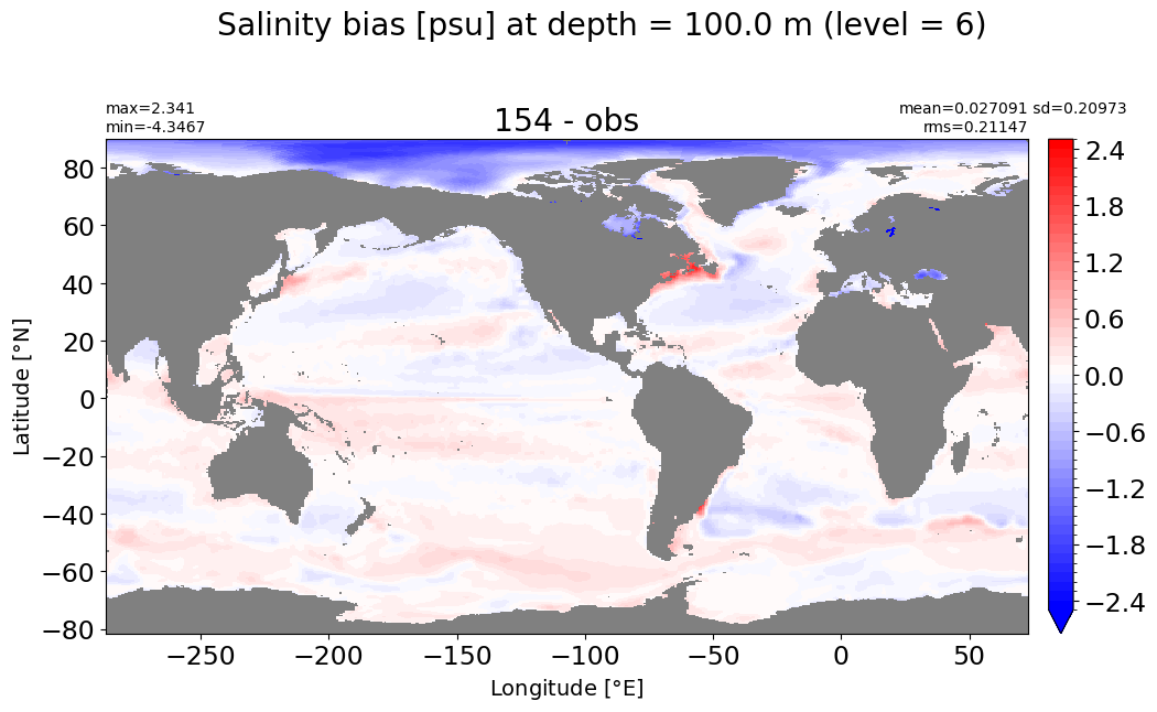
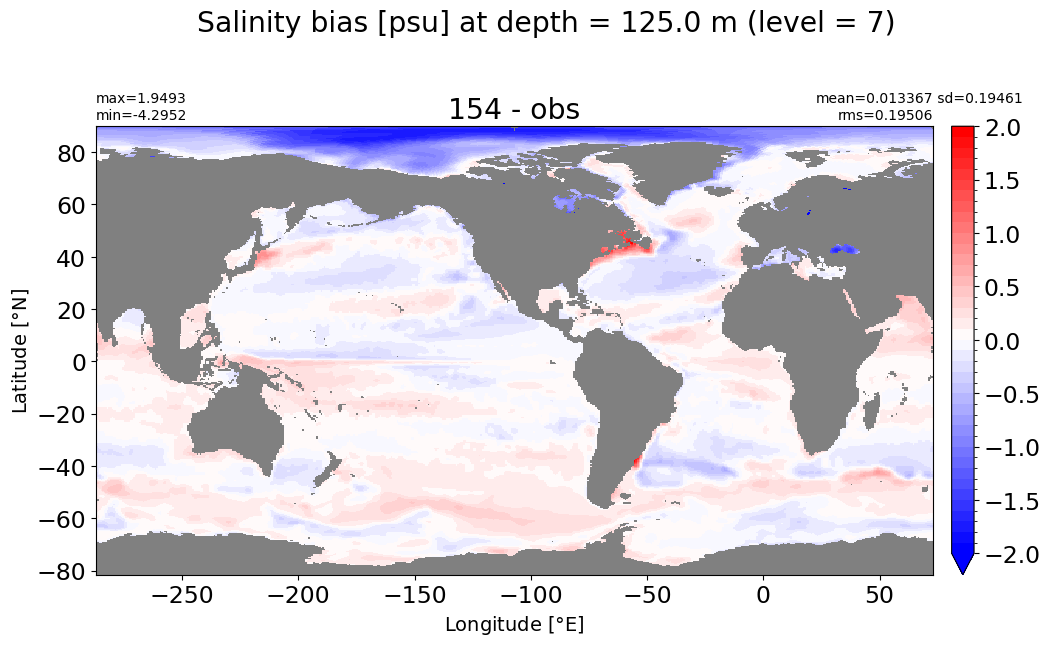
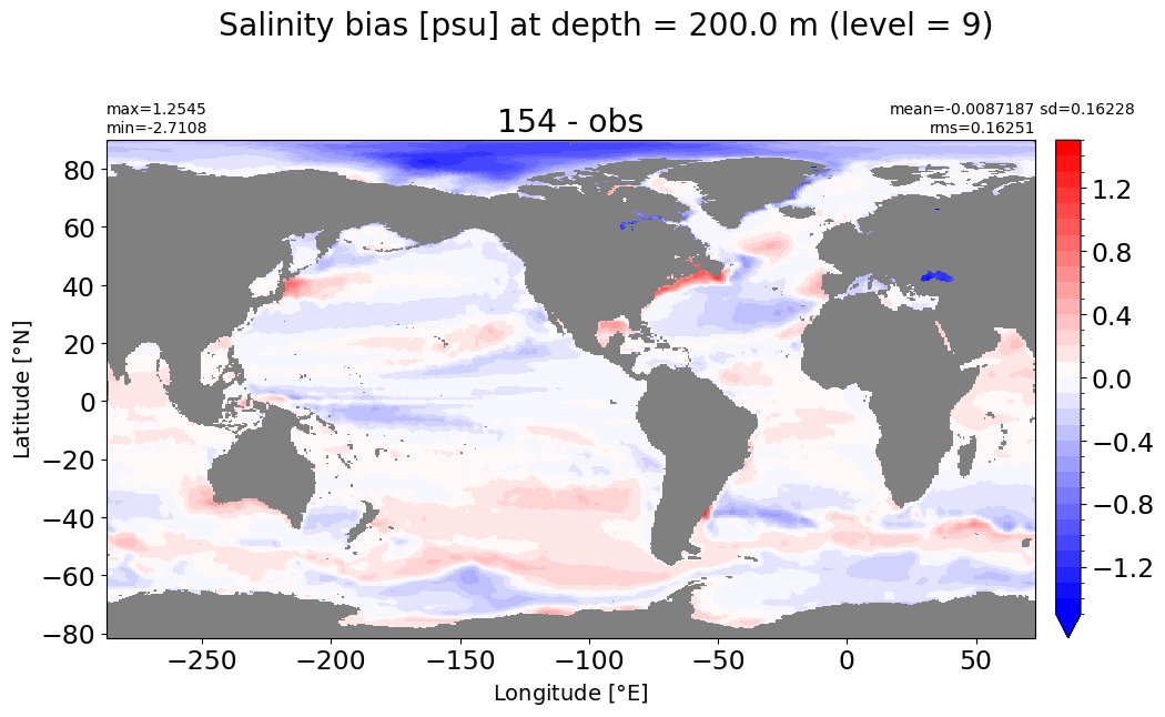
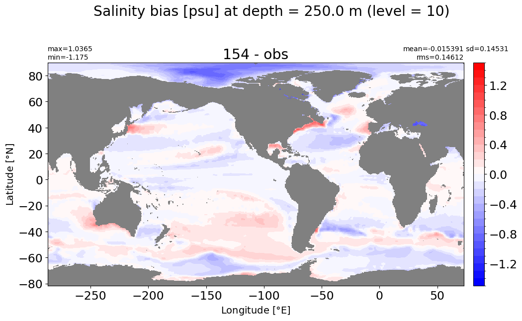
_images/e50fb8414bd2f32848b2715df19046df5c24df130a4224b898d9e758e85bb2ce.png

Salinity#

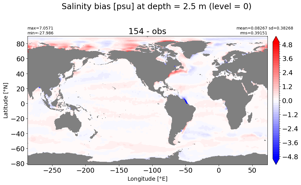
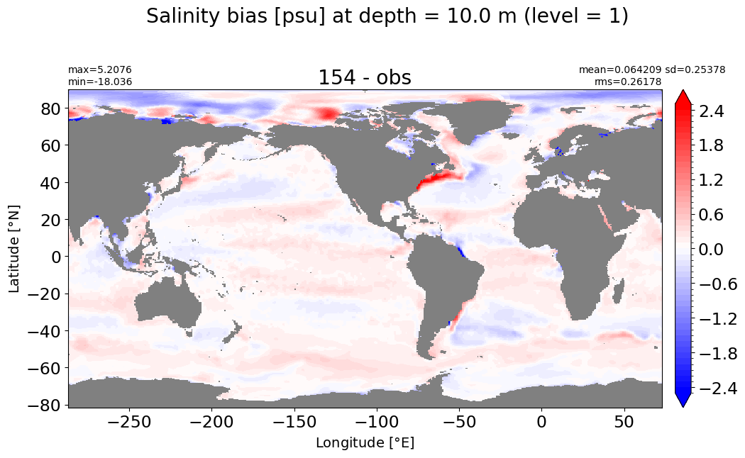
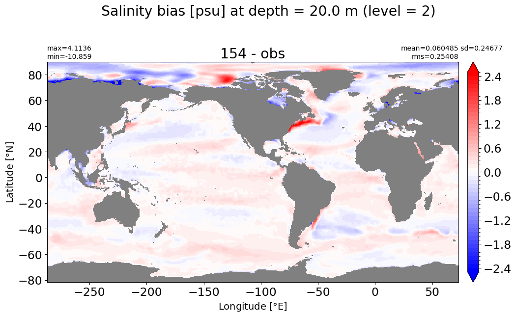
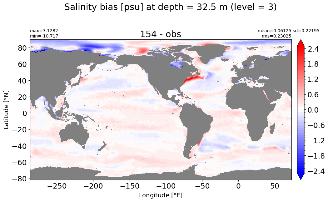
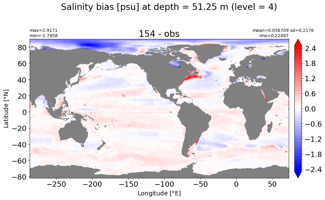
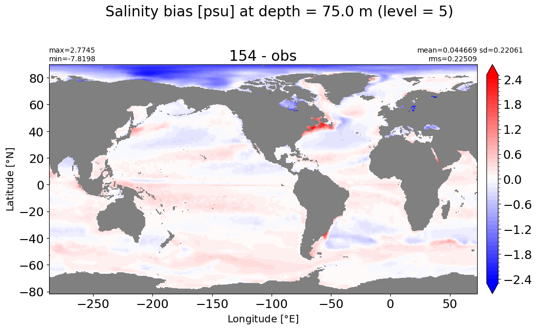
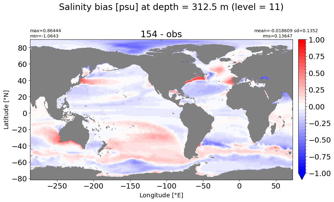
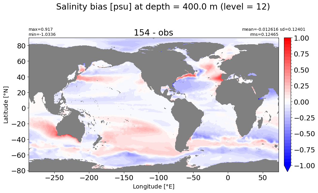
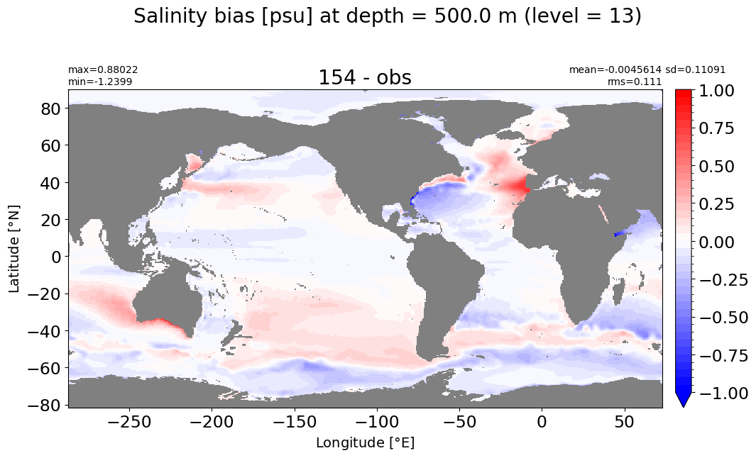
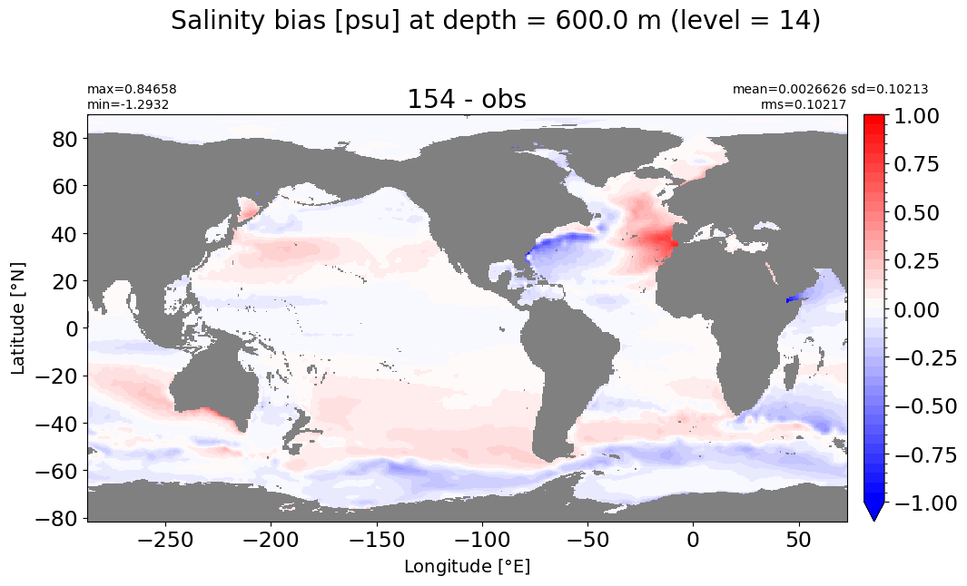
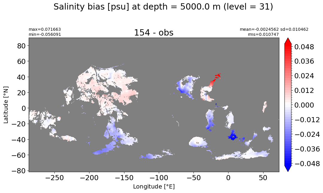
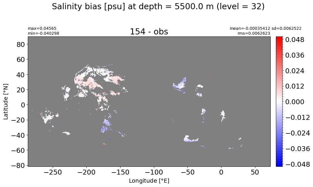
def make_salt_level_plot(k=0, s=5):
    for path, case, i in zip(ocn_path, casename, range(len(casename))):
        if 'area_t' in dir(grd[i]):
          area = grd[i].area_t
        else:
          area = grd[i].areacello
        
        ds_mom_s = xr.open_dataset(path+case+'_so_time_mean.nc')
        fig, ax = plt.subplots(nrows=1, ncols=1, figsize=(12,6.5))
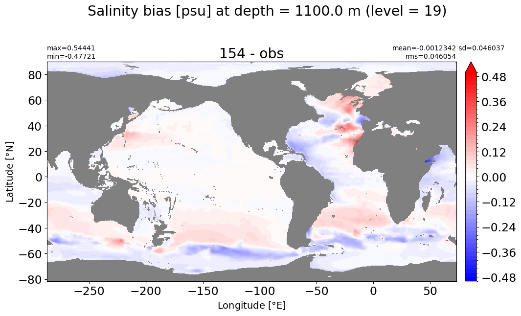
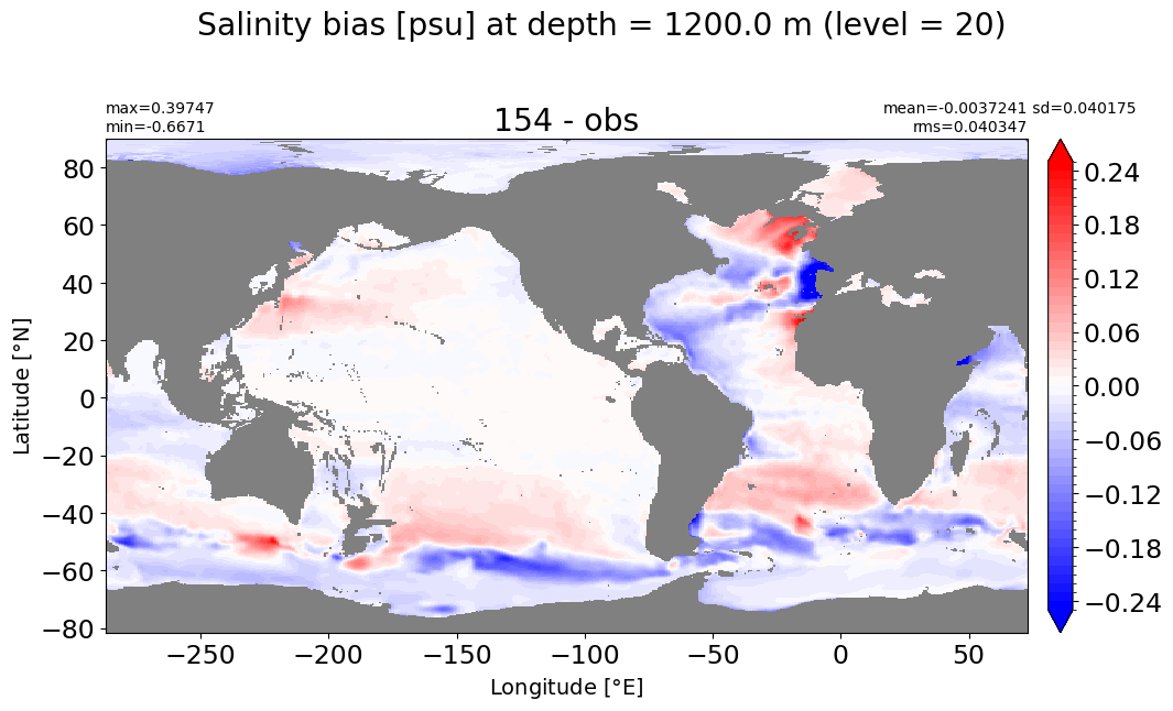
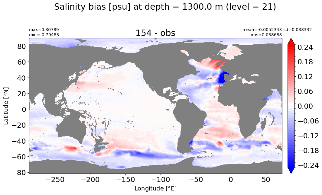
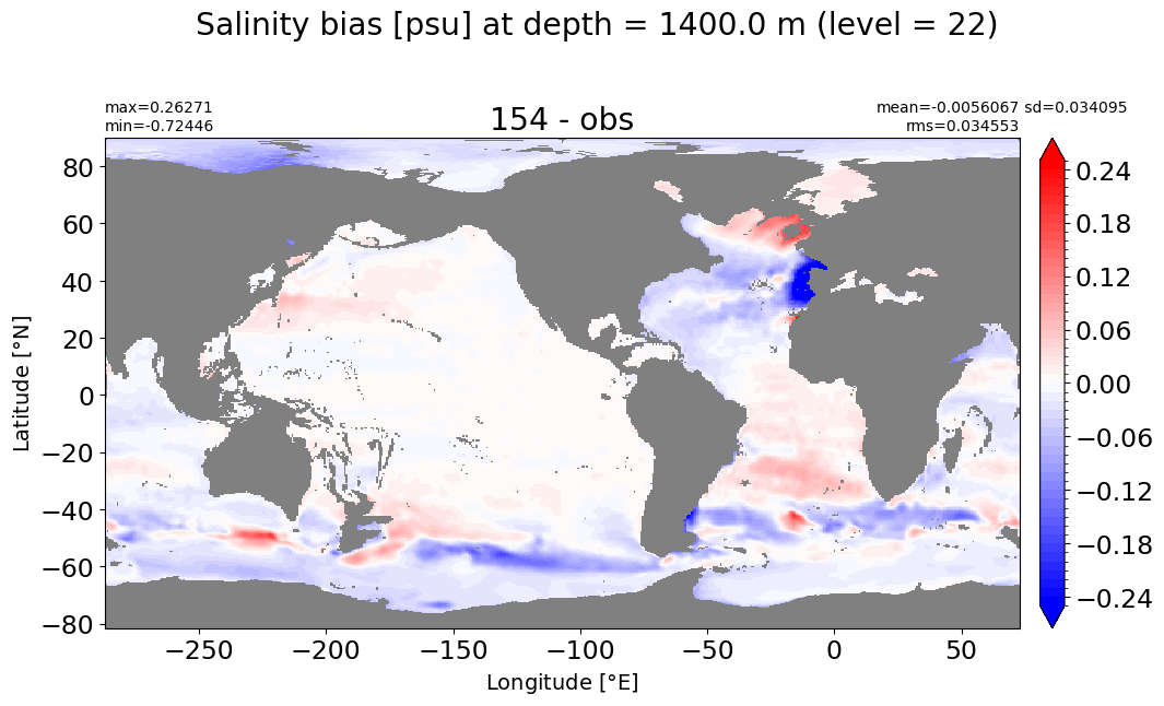
        salt_mom = np.ma.masked_invalid(ds_mom_s.so_bias[k,:].values)
        
        plt.suptitle('Salinity bias [psu] at depth = {} m (level = {})'.format(ds_mom_s.z_l[k].values, k))
        xyplot(salt_mom, grd[i].geolon, grd[i].geolat, area, title=str(label[i]+' - obs'), axis=ax, 
             clim=(-s,s), nbins=50, colormap=plt.cm.bwr, centerlabels=True)
        plt.subplots_adjust(top = 0.8)
    return

Depth = 2.5 m, k=0#

make_salt_level_plot(k=0, s=5)

_images/01933b39cf720a8297a5ce4e4e5c176318c7b41352c823b34b8534db3bd3c411.png

Depth = 10 m, k=1#

make_salt_level_plot(k=1, s=2.5)

_images/c5e8e4e1657d109c3118854d27bff563123fc7f892934d4a912b6569baef6249.png

Depth = 20 m, k=2#

make_salt_level_plot(k=2, s=2.5)

_images/fc06cece95291e4aaac7906b70723e5fdb3d8cb64be5bf53f4c580bb4ad65138.png

Depth = 32.5 m, k=3#

make_salt_level_plot(k=3, s=2.5)

_images/25fe8ae3588b4ee311eddf77d4eb7063b174eeb2b8a49cf07f2d887fabd9371f.png

Depth = 51.25 m, k=4#

make_salt_level_plot(k=4, s=2.5)

_images/523df59e27a5468a2ff291e758014ea83430f4487d718b8c3c451b468c3b9ea5.png

Depth = 75 m, k=5#

make_salt_level_plot(k=5, s=2.5)

_images/f76bf5c89a3015540e2c55f23d3afe5627296179a1a76f09870a73b906c6084f.png

Depth = 100 m, k=6#

make_salt_level_plot(k=6, s=2.5)

_images/69410eee9552fb9e7ad9c648d686d49dc7a9f677c6225f80391f1cb80641959d.png

Depth = 125 m, k=7#

make_salt_level_plot(k=7, s=2.)

_images/11d026bf0ae09099157e58ecfa65f8b374e7b67cdff8148a587238a496f1bd24.png

Depth = 200 m, k=9#

make_salt_level_plot(k=9, s=1.5)

_images/3877eb13f5ba0a7d843447c1792f46e5a322786a00bf61c69110d81626d5d236.png

Depth = 250 m, k=10#

make_salt_level_plot(k=10, s=1.5)

_images/7e35f96bbfa55eccb4319bc3b4e161535a426f6a5cc5d8cfce0721c1448a974e.png

Depth = 312.25 m, k=11#

make_salt_level_plot(k=11, s=1.)

_images/bf6112aeff0e908842d0a6e6bca0b68b0a9cf0a938ec6b38aef201d96e2ae48d.png

Depth = 400 m, k=12#

make_salt_level_plot(k=12, s=1.)

_images/6f2320a8ab17059c7745f040d2f93b6e73d9f2bda597cf52f28b1014b5d9c00a.png

Depth = 500 m, k=13#

make_salt_level_plot(k=13, s=1.)

_images/d6c4dd41c6344f29fa5ac6d92c13fbba22bf2909a59f629a3538d16cd86d5e6b.png

Depth = 600 m, k=14#

make_salt_level_plot(k=14, s=1.)

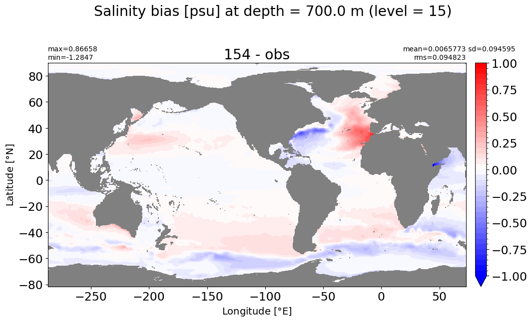
_images/2d3887e856fd03435fdb24daafea89935e1f2244dec840f836f8cad9f1f8f0a2.png

Depth = 700 m, k=15#

make_salt_level_plot(k=15, s=1.)

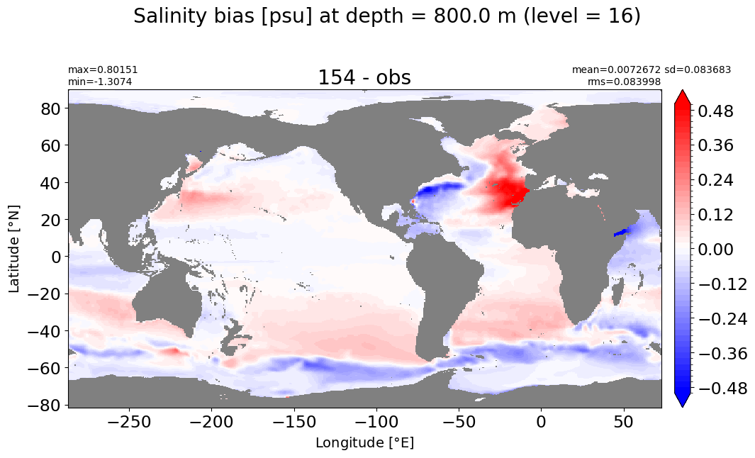
_images/692c1db82cf9accac1fc4fd069f4e5d42368fd9f576846913c6d6f22a0442f65.png

Depth = 800 m, k=16#

make_salt_level_plot(k=16, s=0.5)

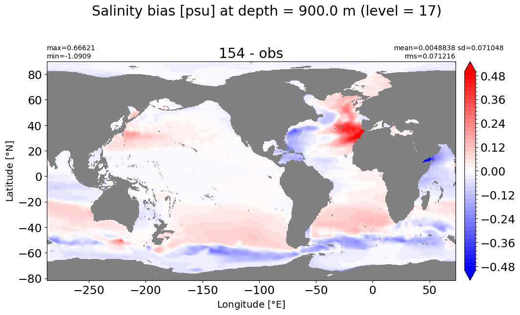
_images/745cd18abc59b462820caf1c5a4ee0ab13362af99b81fbd27ed937cb5b94729c.png

Depth = 900 m, k=17#

make_salt_level_plot(k=17, s=0.5)

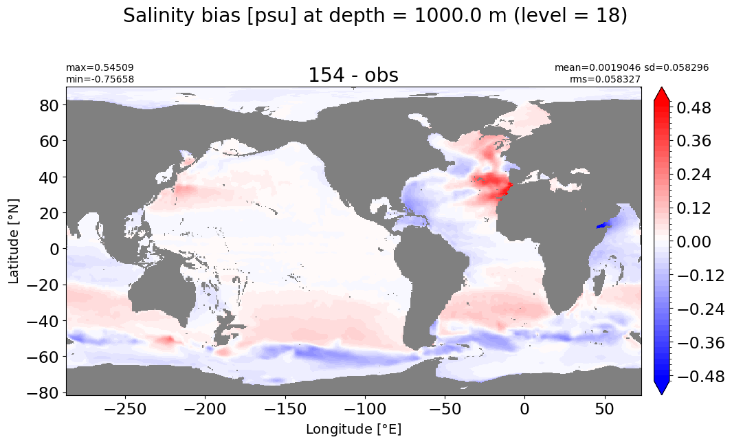
_images/4dc709ce982d61505d1fadd6d12e3c5b787bb63d05fa69517baa23906a9a6a4b.png

Depth = 1000 m, k=18#

make_salt_level_plot(k=18, s=0.5)

_images/dee620e0628e58fb860702aa340b0cb244ea2e7bfd4d028da3a760a5922a6834.png

Depth = 1100 m, k=19#

make_salt_level_plot(k=19, s=0.5)

_images/81e565c4d957cc12eccd076fbb5eddc66d8abb9ef7182ae9dfd8e3cc31004594.png

Depth = 1200 m, k=20#

make_salt_level_plot(k=20, s=0.25)

_images/5c84408c249d6e4901ae451911656d6c0e28a9a9b017de939c6a402a6aba04e9.png

Depth = 1300 m, k=21#

make_salt_level_plot(k=21, s=0.25)

_images/c69d36be377d928ac88d472ee4a2bccfc92a4aa05fbe220d9431a6849ec1707f.png

Depth = 1400 m, k=22#

make_salt_level_plot(k=22, s=0.25)

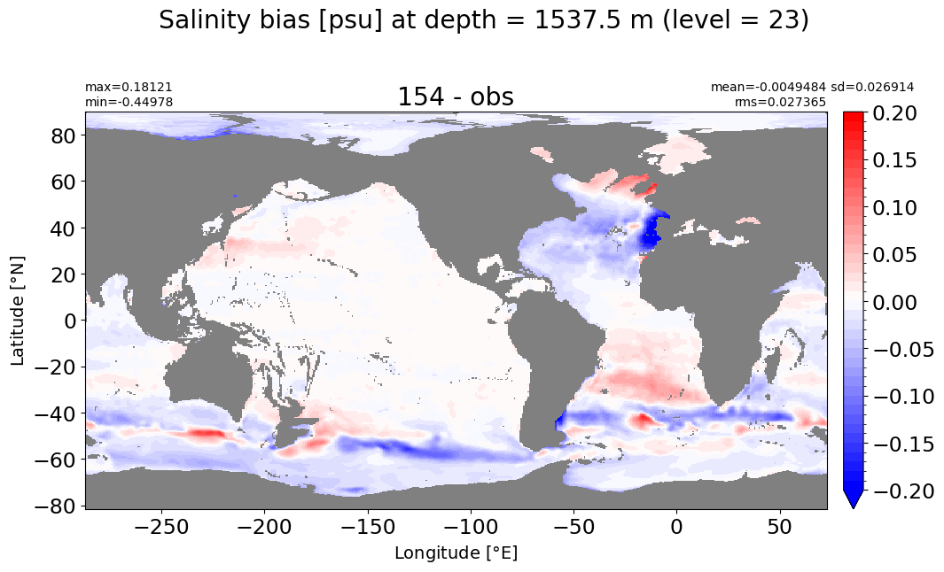
_images/48ed8b95bc67d0e9e2c5a55032406e76a38bac892383a706b3ba1685037a3e89.png

Depth = 1537.5 m, k=23#

make_salt_level_plot(k=23, s=0.2)

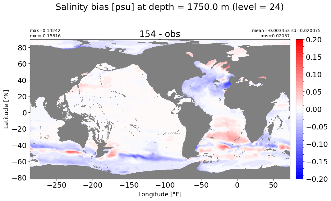
_images/656695aec3b01a24a914fc2a2e50e8b55fab994978fba992e80a203b4ad6c2a7.png

Depth = 1750 m, k=24#

make_salt_level_plot(k=24, s=0.2)

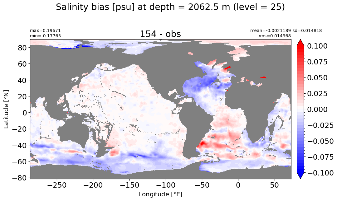
_images/09d194a57008e23aaf23f35269db6ab0918e81f5a8e4a8aa687d9972e1032a1e.png

Depth = 2062.5 m, k=25#

make_salt_level_plot(k=25, s=0.1)

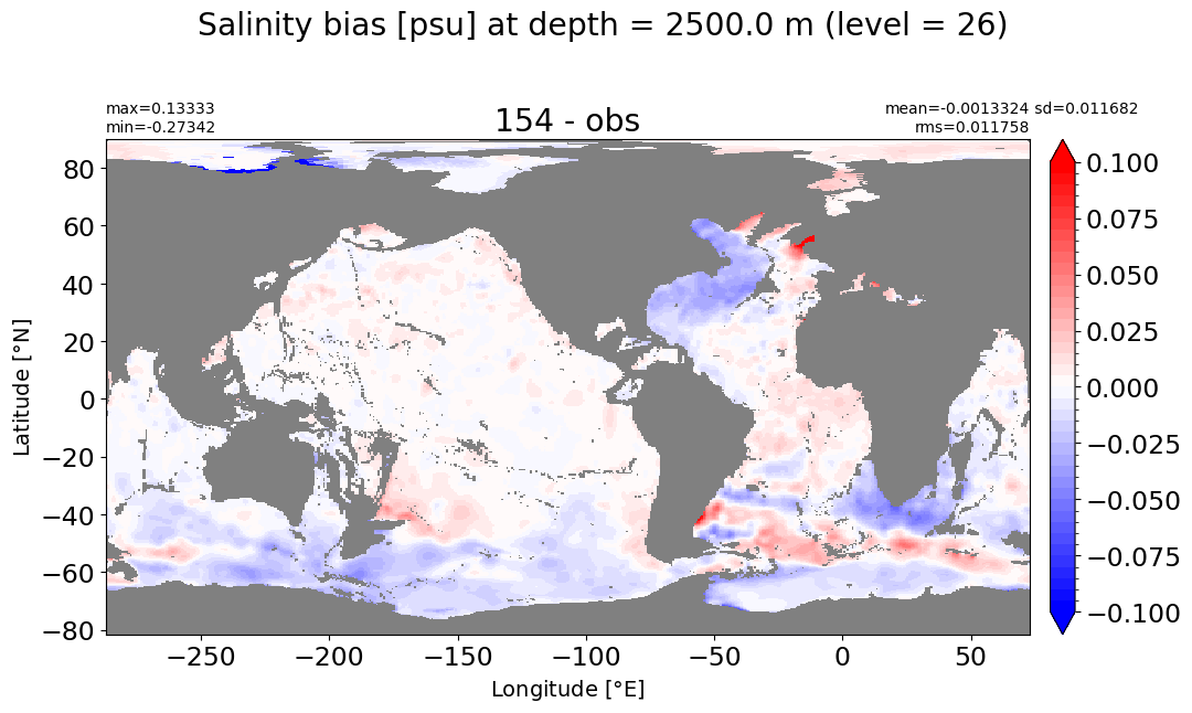
_images/a324aae2eddf616c218ff04054ef4262958c68a7f5fd31659e8dd0adc11ea8dc.png

Depth = 2500 m, k=26#

make_salt_level_plot(k=26, s=0.1)

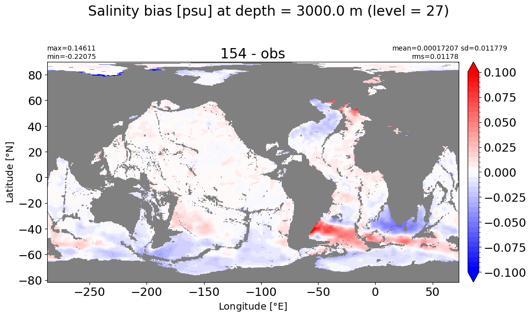
_images/24ec4a5fd742146412415797f89b959ce454a3a82adf6762abb55b85a926e543.png

Depth = 3000 m, k=27#

make_salt_level_plot(k=27, s=0.1)

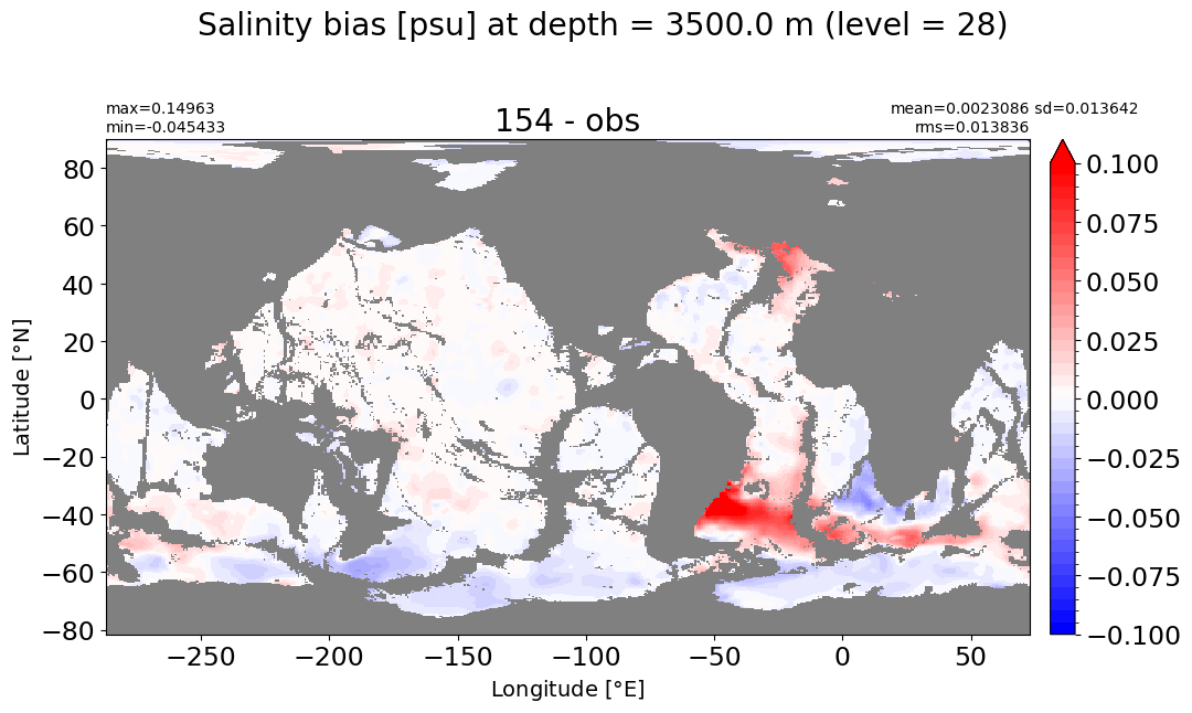
_images/83f466df4aeda9178cd9b555e285bac334e8ece0205f3e82c0f3a3ebfb7378ae.png

Depth = 3500 m, k=28#

make_salt_level_plot(k=28, s=0.1)

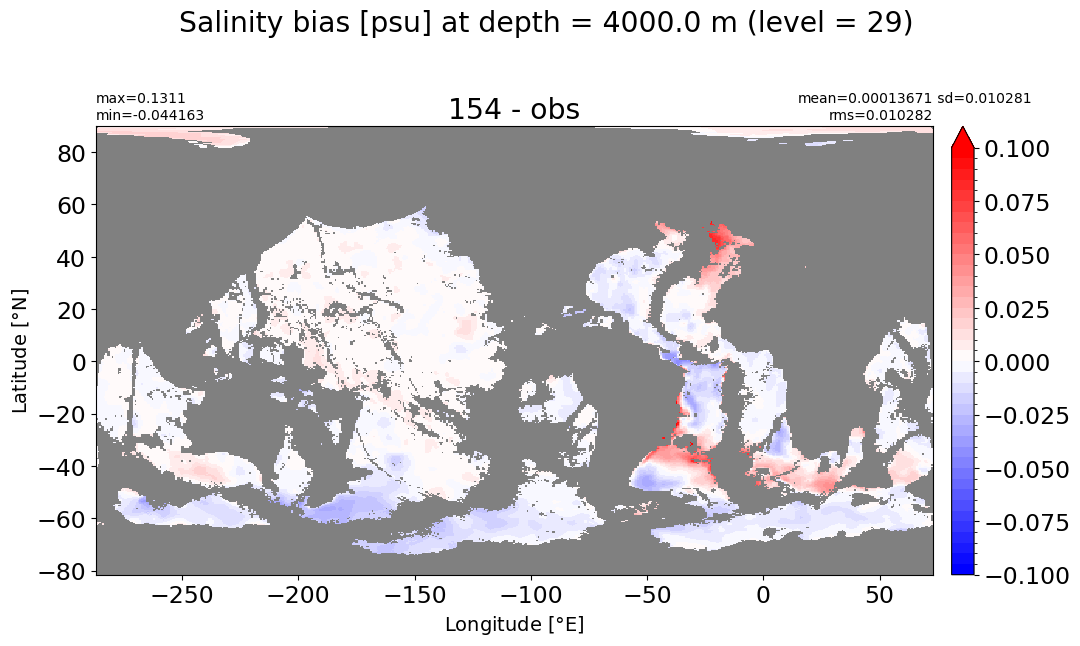
_images/f169598ce7a37443ddab04088a30a909ac182bd1437a20f868c3d6f45c5dd160.png

Depth = 4000 m, k=29#

make_salt_level_plot(k=29, s=0.1)

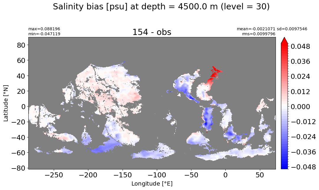
_images/d870a9dcec118b4be93a083f97c90883778cbf63f7819b48dc8eb538e4498c6e.png

Depth = 4500 m, k=30#

make_salt_level_plot(k=30, s=0.05)

_images/3997d455040bf980fc4f19befd389012900e5cb8d23fdaabe76f62b38e537242.png

Depth = 5000 m, k=31#

make_salt_level_plot(k=31, s=0.05)

_images/01d6070d02082ca3ad7bc38258afd082ac312dd8c761085a7a9dd6b681b9ea0b.png

Depth = 5500 m, k=32#

make_salt_level_plot(k=32, s=0.05)

_images/30fbcdaf038fdbff22e8745c56fba995accd4b8e463332c6ef6e9c8a94e5533b.png

Zonal biases#

reg_mom = ['Global', 'PersianGulf', 'RedSea', 'BlackSea', 'MedSea', 'BalticSea',
           'HudsonBay', 'Arctic', 'PacificOcean', 'AtlanticOcean', 'IndianOcean',
           'SouthernOcean', 'LabSea', 'BaffinBay', 'EGreenlandIceland',
           'GulfOfMexico', 'Maritime', 'SouthernOcean60S']

Potential temperature#

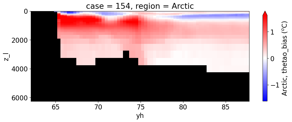
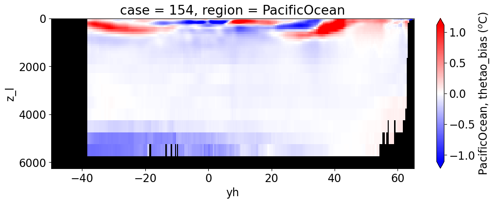
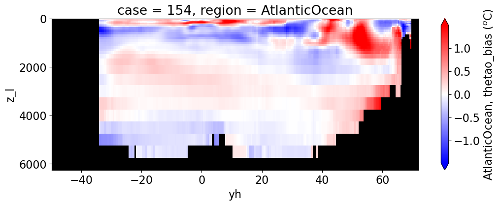
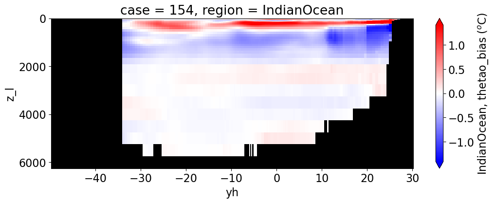
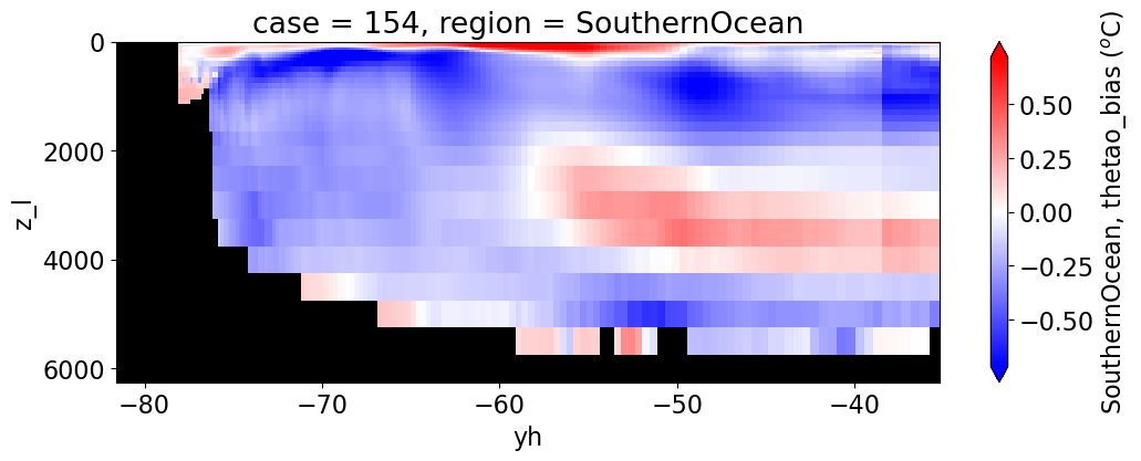
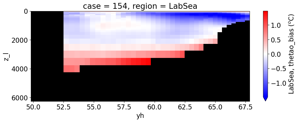
reg = "AtlanticOcean"
var = 'thetao_bias'
units = r'$^o$C'
regions = ['Global','MedSea','Arctic','PacificOcean',
           'AtlanticOcean','IndianOcean','SouthernOcean',
          'LabSea']
ylim_min = [-90, 30, 62, -50, -50, -50, -90, 50]
ylim_max = [ 90, 47, 90,  65,  72,  30, -35, 68 ]

cmap = plt.get_cmap('bwr')  
cmap.set_bad(color='black')  
matplotlib.rcParams.update({'font.size': 16})

for reg, j in zip(regions, range(len(regions))):
  da  = []
  for path, case, i in zip(ocn_path, casename, range(len(casename))):
    ds_mom_t = xr.open_dataset(path+case+'_thetao_time_mean.nc')
    atl = basin_code[i].sel(region=reg)
    # Set zero values to NaN
    atl = atl.where(atl != 0, np.nan)
    da.append((ds_mom_t[var] * atl).weighted(grd_xr[i].areacello.fillna(0)).mean('xh').expand_dims(case=[label[i]]).sel(yh=slice(ylim_min[j], 
                                                                                                                                 ylim_max[j])))

  combined_da = xr.concat(da, dim="case")
  col = None
  if len(combined_da) > 1:
      col = "case"
  g = combined_da.plot(x="yh", y="z_l", col=col, 
                 yincrease=False, col_wrap=2,
                figsize=(12,4), cmap=cmap, robust=True,
                cbar_kwargs={"label": reg + ', ' + var + ' ({})'.format(units)})

_images/e35e5f04d6b14c40f3e5355d354ac0bb031377e0bdaa74bffa072fa04f87c1b2.png

_images/8a13a4b4e39edec721a8ea4b51706cb3867ba1afa33443d0c38d670f61b52339.png

_images/ed9e3bb74253789e847544a6263c2aea88152e26901fd6a6bab0aaf4144acb28.png

_images/619c2df4bd0868b838972f6de153cda69e9e487986ed778ab5103a5a79846292.png

_images/c7b8cde74e1e0b93f8c8ee7e12c3f539ebe1f5a88f2e21e590d404bd063eee02.png

_images/3d8569b705663138f682c4c22fd4565179bc706bd7bfdc6cfca901213dc19eb2.png

_images/9e2d98eb17df917963f49f45d505bbd9bb029f95c90d419d002dbe2c08282e5f.png

_images/6e59ade2a7a2bb4ec0b4a23d38ff569f496dfde5f0826af157ac232b2214c62c.png

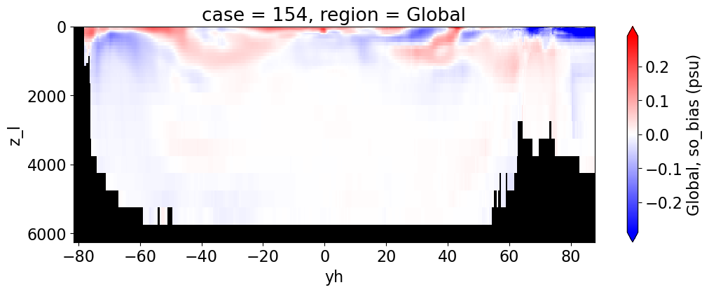
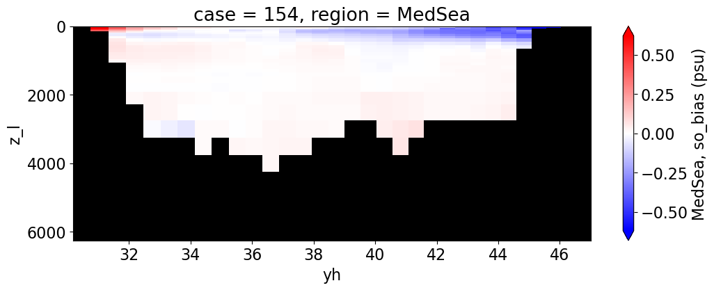
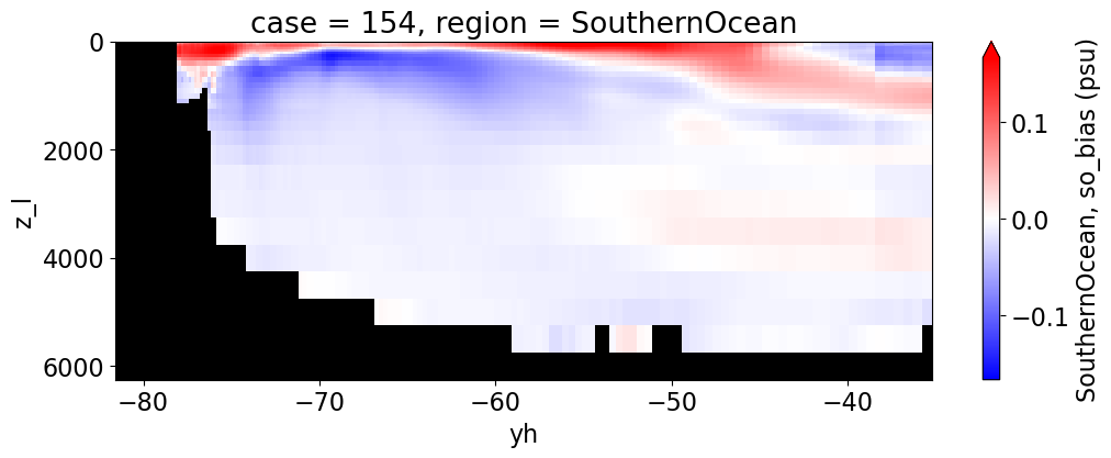
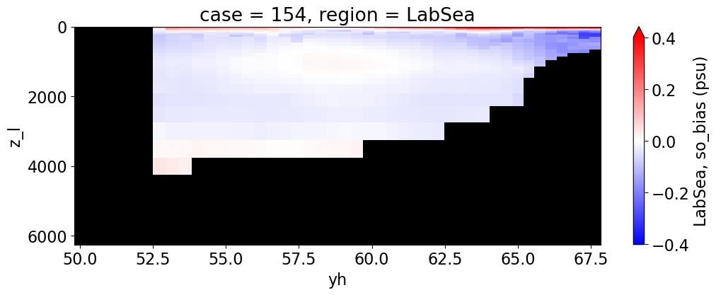
Salinity#

reg = "AtlanticOcean"
var = 'so_bias'
units = 'psu'
regions = ['Global','MedSea','Arctic','PacificOcean',
           'AtlanticOcean','IndianOcean','SouthernOcean',
          'LabSea']
cmap = plt.get_cmap('bwr')  
cmap.set_bad(color='black')  
matplotlib.rcParams.update({'font.size': 16})

for reg, j in zip(regions, range(len(regions))):
  #print(reg)
  da  = []
  for path, case, i in zip(ocn_path, casename, range(len(casename))):
    ds_mom_t = xr.open_dataset(path+case+'_so_time_mean.nc')
    atl = basin_code[i].sel(region=reg)
    # Set zero values to NaN
    atl = atl.where(atl != 0, np.nan)
    da.append((ds_mom_t[var] * atl).weighted(grd_xr[i].areacello.fillna(0)).mean('xh').expand_dims(case=[label[i]]).sel(yh=slice(ylim_min[j], ylim_max[j])))

  combined_da = xr.concat(da, dim="case")
  col = None
  if len(combined_da) > 1:
      col = "case"
  g = combined_da.plot(x="yh", y="z_l", col=col, 
                 yincrease=False, col_wrap=2,
                figsize=(12,4), cmap=cmap, robust=True,
                cbar_kwargs={"label": reg + ', ' + var + ' ({})'.format(units)})

_images/33372bd030f2ea63f9e53aa97407b7311c199a031894ab1f0c160a896b52a155.png

_images/45b9a512c76cb9d9e523598c347f937d0f56dd1408de0bba01eb308ac15e4277.png

_images/6fc9b5f5562f91f687de32e242852c50c22d0762a809ac5407b870455ca8f018.png

_images/ee0390057ac6e945b01b9d43e8d21a6a4e8b0380d100e819cd090d85111a672a.png

_images/163327fdd903f861860e8fa3d4d8ec92db858121e2b29690a4ece0d498758288.png

_images/8afb03d79b9e3743de215a8fb8243c0f50589ce028a0e1fc64f8a5be4342d4ce.png

_images/ef6034e3f9546c28a1b0e7215a51b195556a75971a3a14b269b06678e17b8d4e.png

_images/d097f8442b9b21c5b3862800758496284a55d0b77c0da87c2414b00a5ff16936.png

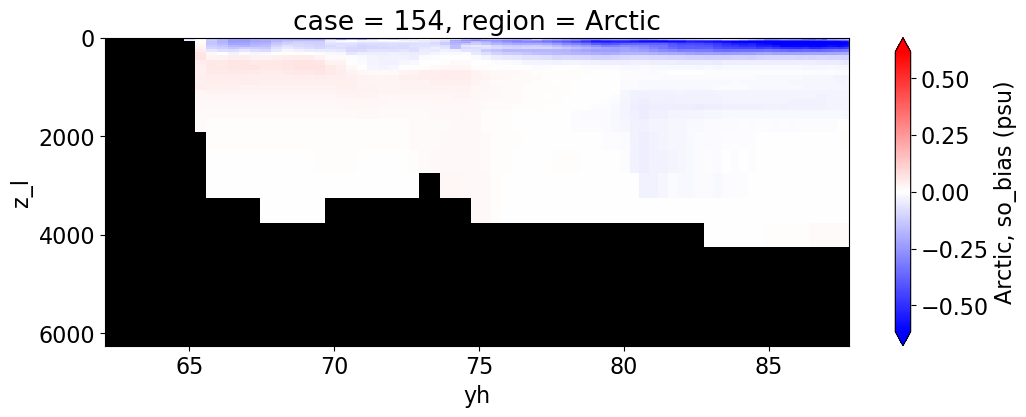
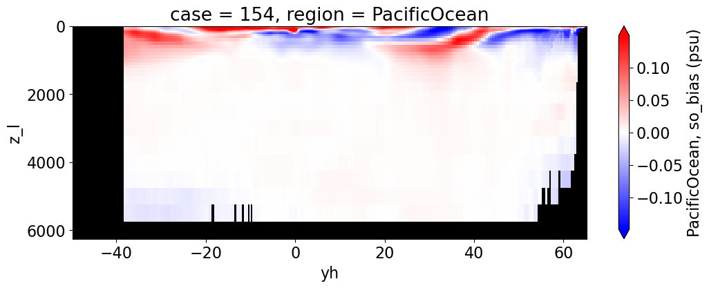
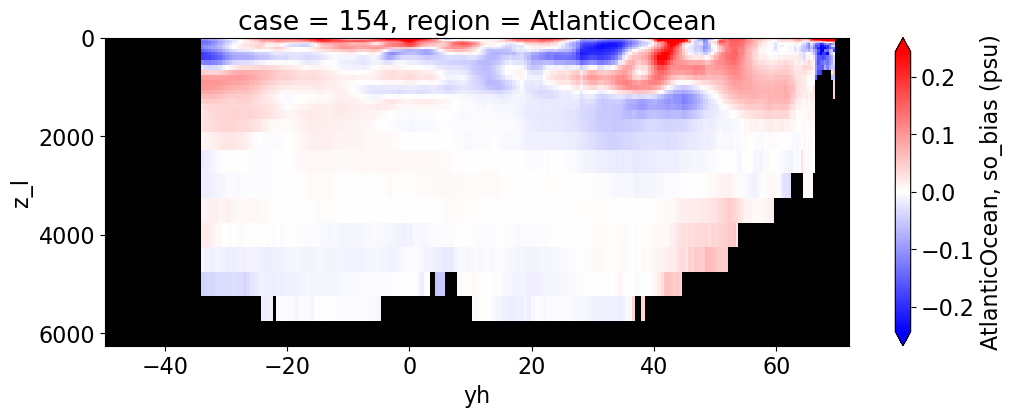
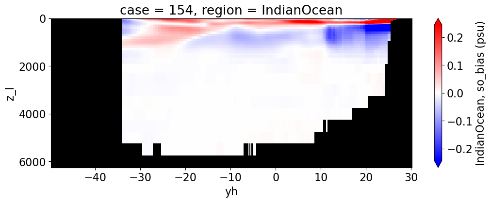
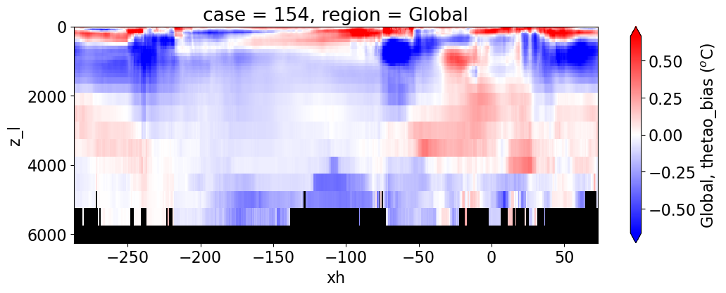
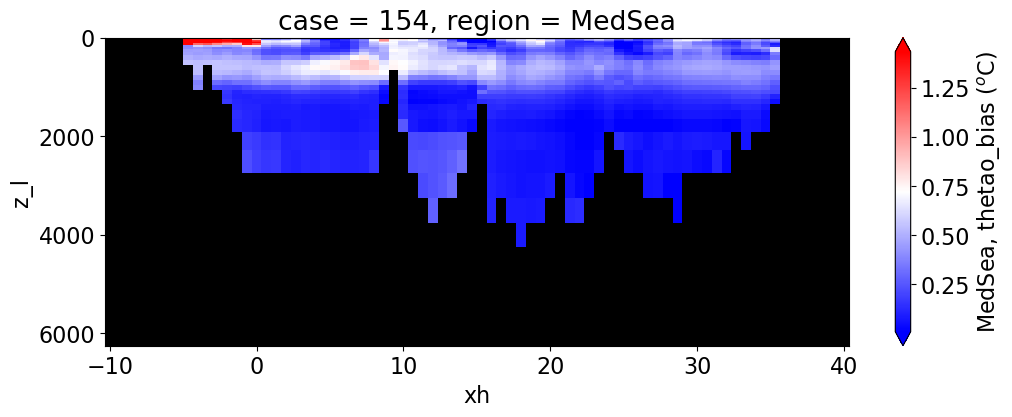
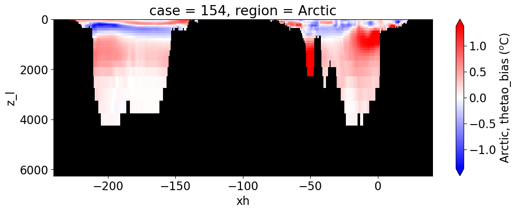
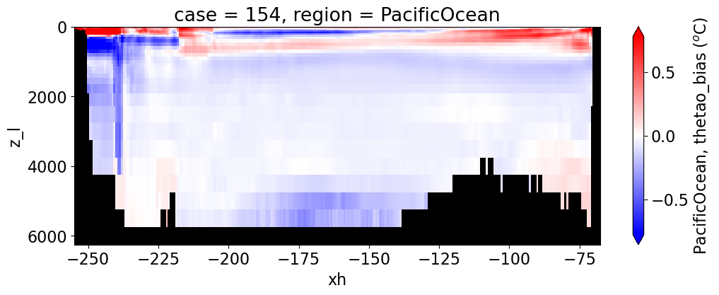
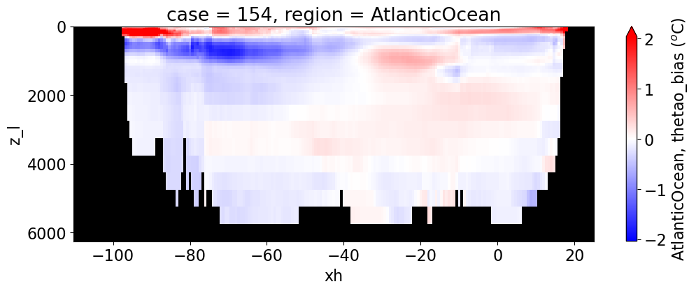
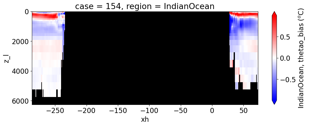
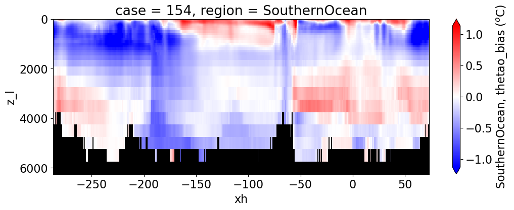
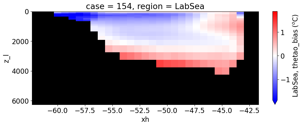
Meridional biases#

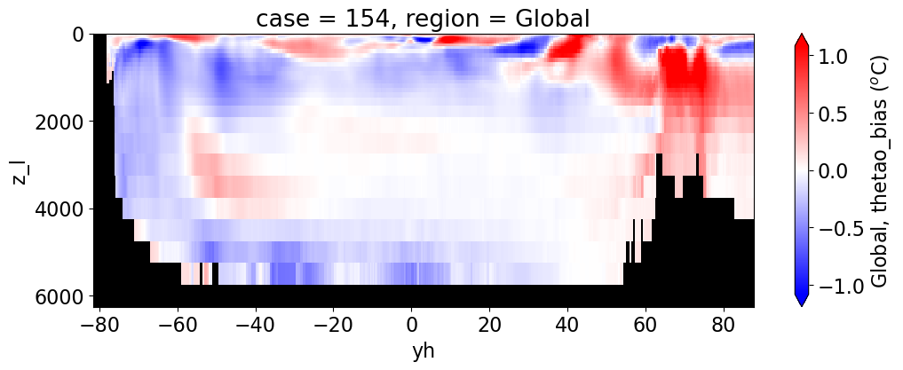
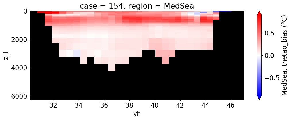
Potential temperature#

reg = "AtlanticOcean"
var = 'thetao_bias'
units = r'$^o$C'
regions = ['Global','MedSea','Arctic','PacificOcean',
           'AtlanticOcean','IndianOcean','SouthernOcean',
          'LabSea']
xlim_min = [-287, -10, -240, -255, -110, -287, -287, -62]
xlim_max = [ 73,   40,   40,  -68,  25,  73, 73, -42 ]
cmap = plt.get_cmap('bwr')  
cmap.set_bad(color='black')  
matplotlib.rcParams.update({'font.size': 16})

for reg, j in zip(regions, range(len(regions))):
  #print(reg)
  da  = []
  for path, case, i in zip(ocn_path, casename, range(len(casename))):
    ds_mom_t = xr.open_dataset(path+case+'_thetao_time_mean.nc')
    atl = basin_code[i].sel(region=reg)
    # Set zero values to NaN
    atl = atl.where(atl != 0, np.nan)
    da.append((ds_mom_t[var] * \
      atl).weighted(grd_xr[i].areacello.fillna(0)).mean('yh').expand_dims(case=[label[i]]).sel(xh=slice(xlim_min[j], 
                                                                                                xlim_max[j])))

  combined_da = xr.concat(da, dim="case")
  col = None
  if len(combined_da) > 1:
      col = "case"
  g = combined_da.plot(x="xh", y="z_l", col=col, 
                 yincrease=False, col_wrap=2,
                figsize=(12,4), cmap=cmap, robust=True,
                cbar_kwargs={"label": reg + ', ' + var + ' ({})'.format(units)})

_images/8b6644d242f6dbd6f8730c4435077323546b7defe60f27f83c2985fa9ef7e8a1.png

_images/dc0d97af33279b0223e7ce26ae08cd751128430cd540669043439dc0cf14cbf1.png

_images/529f3262d8297234a5972776b0292031942cd9fd11e4c7e85409ba9bd41e7bd5.png

_images/909f04ecc6664167c70792ce7bcd7a447304834dc5a65a25d5d696cfc785d3e7.png

_images/5e9d6e3b53b8fc7c33a6bd185e9bc29d34f8b06d4afb5777f6a69e950013b25f.png

_images/bf9412f26886d56991cf070694583171484eaa654659e3b8ea4a1e07ed17faa1.png

_images/082242f6a2b4841f3ed3b81ca4fef5ae6e422f863158ae971f945b85587541d8.png

_images/815a0b423a6463d1940b0b3a3952ec7316ecf697032e0f3a8e70a3783ee444ce.png

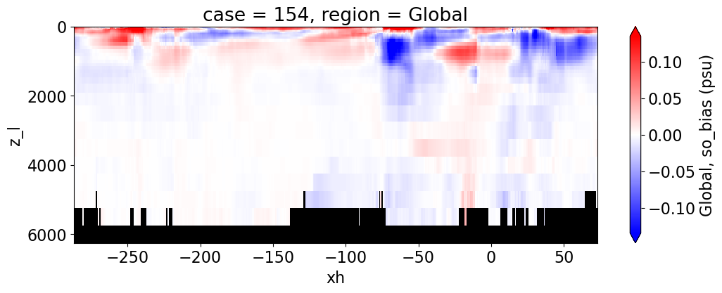
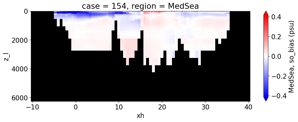
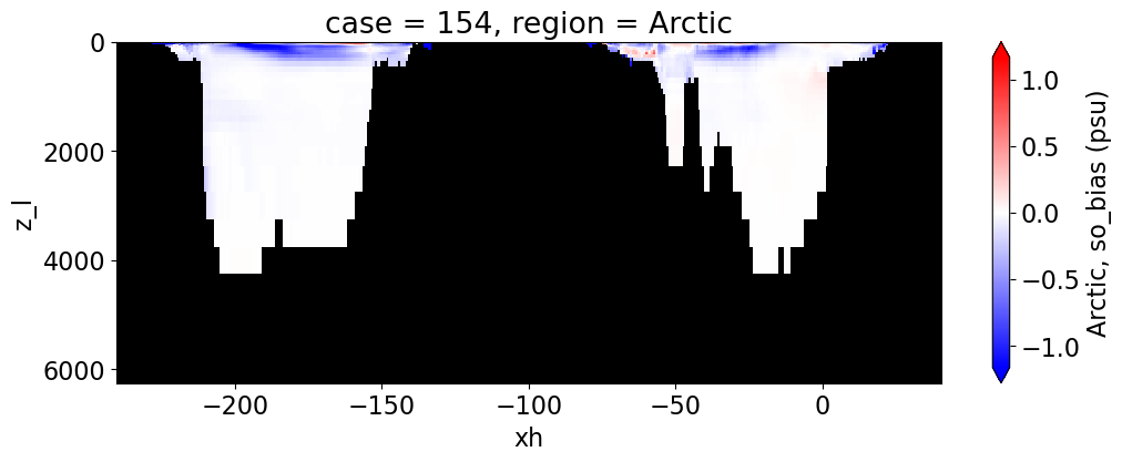
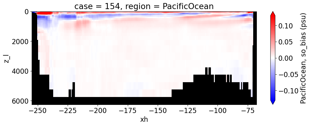
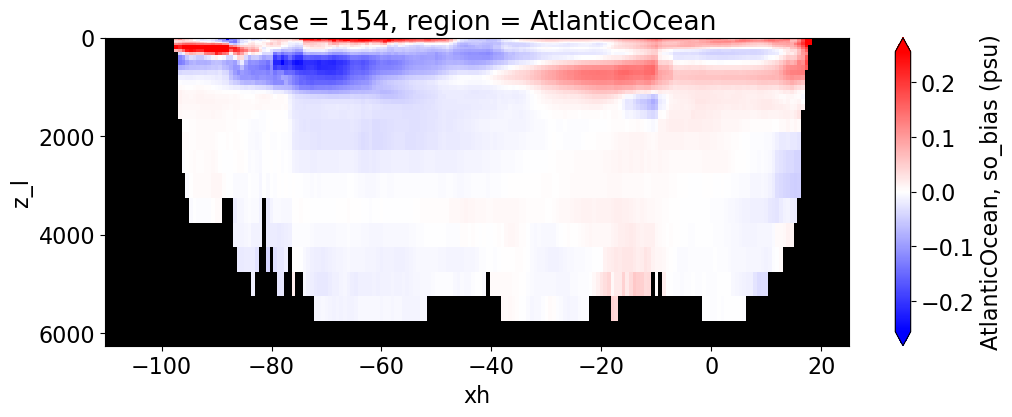
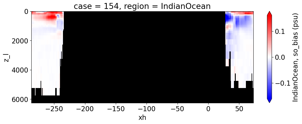
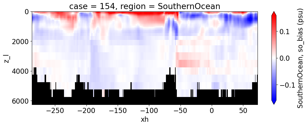
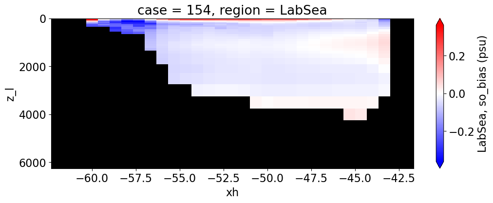
Salinity#

reg = "AtlanticOcean"
var = 'so_bias'
units = 'psu'
regions = ['Global','MedSea','Arctic','PacificOcean',
           'AtlanticOcean','IndianOcean','SouthernOcean',
          'LabSea']
cmap = plt.get_cmap('bwr')  
cmap.set_bad(color='black')  
matplotlib.rcParams.update({'font.size': 16})

for reg, j in zip(regions, range(len(regions))):
  #print(reg)
  da  = []
  for path, case, i in zip(ocn_path, casename, range(len(casename))):
    ds_mom_t = xr.open_dataset(path+case+'_so_time_mean.nc')
    atl = basin_code[i].sel(region=reg)
    # Set zero values to NaN
    atl = atl.where(atl != 0, np.nan)
    da.append((ds_mom_t[var] * \
      atl).weighted(grd_xr[i].areacello.fillna(0)).mean('yh').expand_dims(case=[label[i]]).sel(xh=slice(xlim_min[j], 
                                                                                               xlim_max[j])))

  combined_da = xr.concat(da, dim="case")
  col = None
  if len(combined_da) > 1:
      col = "case"
  g = combined_da.plot(x="xh", y="z_l", col=col, 
                 yincrease=False, col_wrap=2,
                figsize=(12,4), cmap=cmap, robust=True,
                cbar_kwargs={"label": reg + ', ' + var + ' ({})'.format(units)})

_images/de5ae5e76d69a4efc575d11b990b825b6a497c289bd9d9ed521ea4399c9ac624.png

_images/d0d9d675861881f3e16672bb74fb4ae78209d1ec75a090b35d924f7be30600b1.png

_images/fe18e37dfbec602323a37e23201a07092bdadfa6f1652dc400cfc826eb887f07.png

_images/f3fe924348c34f7f86106e249d495a8e2005758490cd43a6beda965f1f4729a6.png

_images/a25973c4355ea0cc9bcab82cf75c2a075baaf83ae5c641c61b1622c8eaa45ba2.png

_images/3f72baadfd4669a5ec4d4622bbe0875aa59322000f04b5374ec490bc123f4217.png

_images/877dfd95386eefa2d4bb2e7a56a9e1fce8eacf9fae99daf039168611b9fe9a87.png

_images/7a812336f9d8b00aa378ff34569e0cb0fbb4a21820577a6fb6126113b88d9cdf.png

T & S biases

Contents

T & S biases#

Drifts#

Potential temperature#

Global#

Arctic#

SouthernOcean#

SouthernOcean60S#

PacificOcean#

AtlanticOcean#

IndianOcean#

Maritime#

BalticSea#

PersianGulf#

RedSea#

BlackSea#

MedSea#

HudsonBay#

LabSea#

BaffinBay#

EGreenlandIceland#

GulfOfMexico#

Salinity#

Global#

Arctic#

SouthernOcean#

SouthernOcean60S#

PacificOcean#

AtlanticOcean#

IndianOcean#

Maritime#

BalticSea#

PersianGulf#

RedSea#

BlackSea#

MedSea#

HudsonBay#

LabSea#

BaffinBay#

EGreenlandIceland#

GulfOfMexico#

RMSE#

Potential Temperature#

Global#

Arctic#

SouthernOcean#

SouthernOcean60S#

PacificOcean#

AtlanticOcean#

IndianOcean#

Maritime#

BalticSea#

PersianGulf#

RedSea#

BlackSea#

MedSea#

HudsonBay#

LabSea#

BaffinBay#

EGreenlandIceland#

GulfOfMexico#

Salinity#

Global#

Arctic#

SouthernOcean#

SouthernOcean60S#

PacificOcean#

AtlanticOcean#

IndianOcean#

Maritime#

BalticSea#

PersianGulf#

RedSea#

BlackSea#

MedSea#

HudsonBay#

LabSea#

BaffinBay#

EGreenlandIceland#